
Neural Networks: Building Blocks
Overview
Artificial neural networks are composed by a variety of functions. This is a collection of my notes on these building blocks. A Jupyter notebook with the code used to generate the illustrations and compute the results is available here.
This is a work in progress. Depth and breadth vary throughout; recent sections are more detailed and expansive than those written at the start. Contributions in the form of errata or suggestions are welcome. Please send me an email or open an issue in the Github repository of this website.
A Single Neuron
Neurons are at the core of artificial neural networks. Like the networks they form, they are inspired by their biological counterparts but are not models of them.
A neuron weighs its inputs separately and passes their sum through an activation function. The result of this operation is the neuron’s activation. Typically, a bias is added to the weighted sum of the inputs to allow a left- or rightward shift of the activation function.
\[y = σ(w_{1}x_{1} + w_{2}x_{2} + w_{3}x_{3} + ... + w_{n}x_{n} + b)\] \[y = σ(\sum\limits_{i=1}^n w_{i}x_{i} + b)\]where the neuron’s activation \(y\) is determined by a sigmoid activation function \(σ\), the neuron’s weights \(w_{n}\), its inputs \(x_{n}\), and a bias \(b\).

The weights and inputs can be represented as tensors and the weighted sum can be therefore computed as a dot product between the weight tensor \(w\) and the input tensor \(x\).
\[y = \sigma(w \cdot x + b)\]One advantage of computing the weighted sum as a dot product is that we can leverage efficient, highly-parallelized libraries such as BLAS (Basic Linear Algebra Subprograms) implementations or parallel computing platforms such as CUDA.
weights = np.array([0.1, 0.2, 0.3])
input = np.array([0.2, 0.3, 0.1])
bias = 1

sum([w * x for w, x in zip(weights, input)]) + bias
1.11
np.dot(input, weights) + bias
1.11
The operation of calculating the output of a neural network based on some input is called a forward pass or, more generally, forward propagation.
class Neuron():

    def __init__(self, weights, bias):
        self.weights = weights
        self.bias = bias

    def forward(self, input):
        """A forward pass through the neuron"""
        z = np.dot(self.weights, input) + self.bias
        print(f"Weighted sum = {z}")
        # Sigmoid activation function
        y = 1 / (1 + math.exp(-z))
        return y

neuron = Neuron(weights, bias)
print(f"Activation = {neuron.forward(input)}")
Weighted sum = [[1.11]] Activation = 0.7521291114395702
Note: Neural networks consisting of a single neuron date back to the 1950s. The perceptron, a machine learning algorithm used for binary classification, effectively consists of a single neuron using a Heaviside step function as its activation function.
Activation Functions
Activation functions are analogous to the action potential in biological neurons. The activation function determines whether a neuron activates and to what extent.
Activation functions allow neural networks to learn layered representations of the input data and account for non-linear relationships.
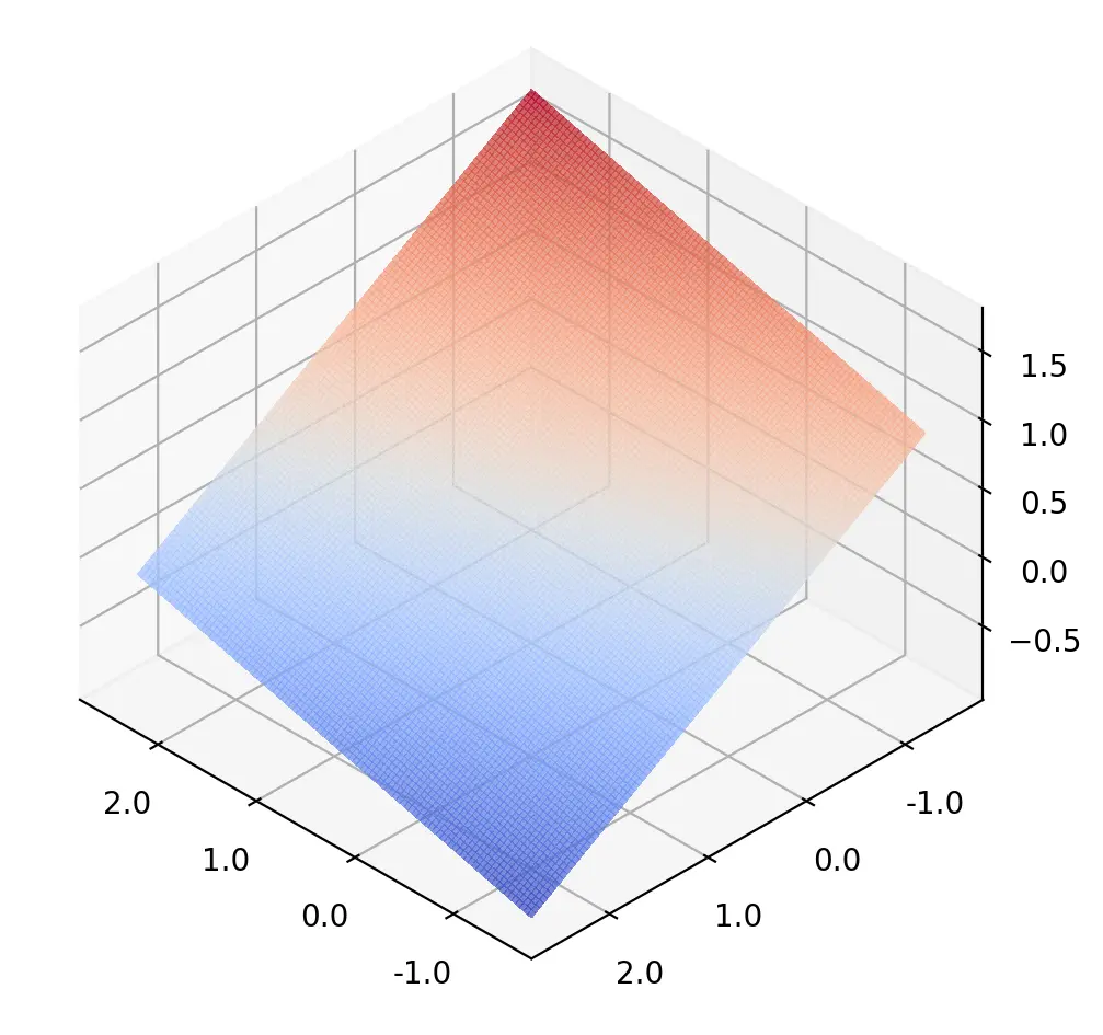
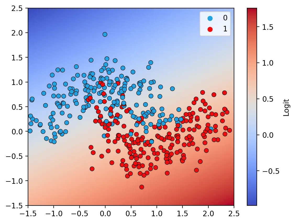
If the output of a neuron were the weighted sum of its inputs, neural networks would simply represent a linear function. Even deep neural networks with several layers could be reduced to a linear function of their input. Linear hyperplanes (constant decision boundaries) are limited representations that are unable to capture nonlinear features.
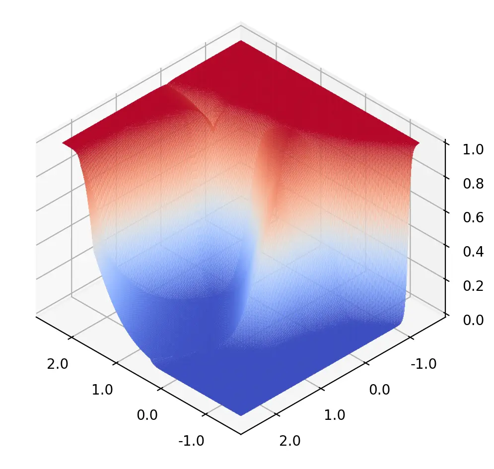
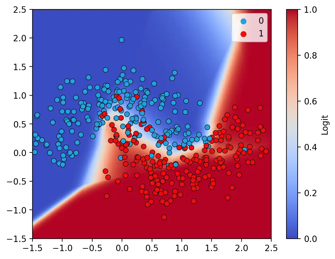
The decision surface illustrated above is that of a model with ReLU and Sigmoid activation functions. This model achieves an accuracy of 91.25% on the training data. In contrast, a model without nonlinear activation functions is only able to learn a linear decision surface, as illustrated below. The linear model is unable to fully capture the features in the training set and achieves an accuracy of only 83.25%.
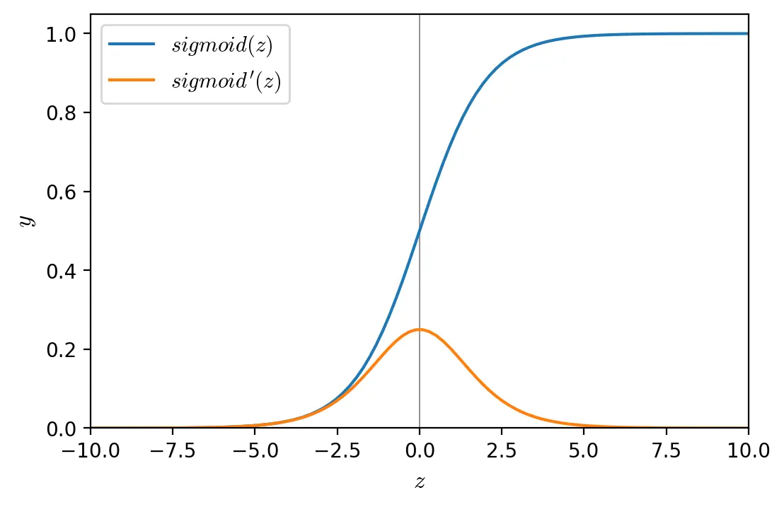
Sigmoid
Sigmoid (also known as logistic function) is a non-linear, continuously differentiable, monotonic activation function. It has a fixed range \((0,1)\). One of the issues with sigmoid is that it is susceptible to the vanishing gradient problem.
\[sigmoid(z) = \dfrac{1}{1 + e^{-z}}\] \[sigmoid'(z) = sigmoid(z)(1-sigmoid(z))\]def sigmoid(z, derivative=False):
"""Sigmoid activation function"""
if derivative:
return sigmoid(z) * (1 - sigmoid(z))
return 1 / (1 + np.exp(-z))
Tanh
Tanh is a non-linear, continuously differentiable activation function that comes from the same family of functions as sigmoid. However, tanh is zero-centered, meaning that the average of its inputs is zero. Zero-centered inputs and activations have been shown to improve the convergence of neural networks during training (see Efficient BackProp by LeCun et al.). Tanh is therefore often preferred to sigmoid, even though it also suffers from the vanishing gradient problem.
\[tanh(z) = \dfrac{e^z - e^{-z}}{e^z + e^{-z}}\] \[tanh'(z) = 1 - tanh(z)^2\]def tanh(z, derivative=False):
"""Tanh activation function"""
if derivative:
return 1 - np.power(tanh(z), 2)
return (np.exp(z) - np.exp(-z)) / (np.exp(z) + np.exp(-z))

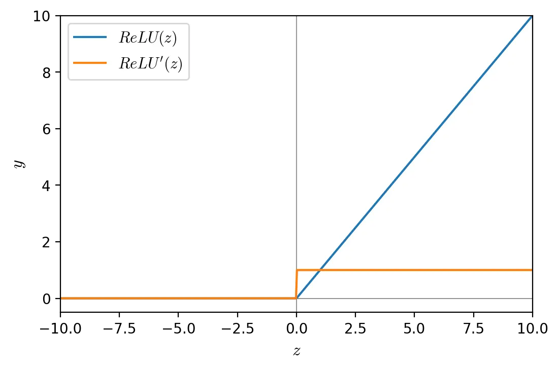
Rectified Linear Unit (ReLU)
ReLU is a non-linear activation function with range \([0, ∞)\). ReLU is less computationally expensive than other activation functions because it involves simpler mathematical operations, and therefore allows for faster training. Moreover neural networks using ReLU benefit from sparse activation: not all neurons in a hidden layer are activated (activation > 0). However, ReLU neurons can suffer from the dying ReLU problem.
\[ReLU(x) = max(0, x)\] \[ReLU'(x)= \begin{cases} 0 & \text{if } x < 0 \\ 1 & \text{if } x > 0 \\ \end{cases}\]def relu(z, derivative=False):
"""ReLU activation function"""
if derivative:
return (z > 0) * 1
return np.maximum(0, z)
A Network of Neurons
Layers
A single neuron can only extract a limited representation on its own. In neural networks, neurons are therefore aggregated into connected layers. Layers extract representations out of the data fed into them and, chained together, progressively distill the data.
All weights in a layer can be represented as a matrix \(W\) with \(k\) neurons, each with \(n\) weights. The sums of the weighted inputs of all neurons in the \(n\)-th layer can be calculated as a the matrix-vector product between the weights matrix and the vector \(a^{(n-1)}\) of the activations of the previous layer. The activation vector \(a^{(n)}\) of the \(n\)-th layer is then the sum of the weighted inputs vector and the bias vector \(b\), passed through an activation function.
\[a^{(n)} = σ \begin{pmatrix} \begin{bmatrix} w_{0,0} & w_{0,1} & \dots & w_{0,n} \\ w_{1,0} & w_{1,1} & \dots & w_{1,n} \\ \vdots & \vdots & \ddots & \vdots \\ w_{k,0} & w_{k,1} & \dots & w_{k,n} \\ \end{bmatrix} \begin{bmatrix} a_{0}^{(n-1)} \\ a_{1}^{(n-1)} \\ \vdots \\ a_{n}^{(n-1)} \\ \end{bmatrix} + \begin{bmatrix} b_{0} \\ b_{1} \\ \vdots \\ b_{n} \\ \end{bmatrix} \end{pmatrix}\] \[a^{(n)} = σ(W^{n}a^{(n-1)} + b^{n})\]# 3 inputs, 2 neurons
input = np.array([[1.4, 0.62, 0.21]]) # (1, 3)
weights = np.array([[0.18, 0.24], [0.32, -0.15], [0.6, -0.28]]) # (3, 2)
biases = np.array([[1, 3]]) # (1, 2)
[relu(sum([x * w for x, w in zip(neuron, input[0])]) + bias) for neuron, bias in zip(weights.T, biases[0])]
[1.5764, 3.1842]
relu(np.sum(input.T * weights, axis=0) + biases)
array([[1.5764, 3.1842]])
relu(np.dot(input, weights) + biases)
array([[1.5764, 3.1842]])
The neural network below has one input layer, one output layer, and two hidden layers. The input layer represents the initial input fed into the network. The hidden layers are the layers between the input and output layers. Hidden and output layers are neural layers that compute activations for their inputs. Output layers sometimes use different activation functions than the hidden layers to return a normalized result (e.g. w/ sigmoid) or a probability distribution (e.g. w/ softmax).

The layers that constitute the network above are fully connected (also called densely connected), meaning that each neuron in a layer is connected to all neurons from the previous layer. Models made up of fully connected layers are called fully connected neural networks (FCNN). In contrast, in other neural networks such as convolutional neural networks (CNN), neurons are only connected to a small region of the previous layer.
Batches
A forward pass can also be performed on a data batch, i.e. a collection of samples. The first axis of a batch tensor is called the batch axis or batch dimension.
inputs = np.array([
    [1.4, 0.62, 0.21], # Sample 1
    [1.4, 0.62, 0.21], # Sample 2
])
inputs.shape
(2, 3)
A batch can be processed in a single forward pass through a layer.
relu(np.dot(inputs, weights) + biases)
array([[1.5764, 3.1842], [1.5764, 3.1842]])
Numpy’s matmul function and its equivalent @ operator are identical to the dot function when the weight and input tensors have 2 or less dimensions. However, when the number of dimensions of either tensor is greater than 2, matmul and @ broadcast stacks of matrices together as if the matrices were elements.
relu(inputs @ weights + biases)
array([[1.5764, 3.1842], [1.5764, 3.1842]])
Matrix multiplication on a data batch is significantly faster than calculating the dot product on each individual sample and only marginally slower than calculating it for a single sample.
%timeit [relu(input @ weights + biases) for input in inputs]
8.6 µs ± 552 ns per loop (mean ± std. dev. of 7 runs, 100000 loops each)
%timeit relu(inputs @ weights + biases)
4.01 µs ± 569 ns per loop (mean ± std. dev. of 7 runs, 100000 loops each)
inputs = inputs[0]
%timeit relu(inputs @ weights + biases)
3.9 µs ± 634 ns per loop (mean ± std. dev. of 7 runs, 100000 loops each)
Networks and Graphs
Neural networks can be represented at different levels of abstraction. The perspective taken so far is that they are a chain of layers and that each layer represents a set of neurons. However, this point of view is reductive. Layers are an abstraction and not a fundamental building block. The core unit of neural networks are functions of one or more variables. A layer can thus represent any combination of one or more functions.
A neural network can be formally described as a computational graph. The network is thus a directed graph where every node is a variable (e.g. scalar, tensor, etc.) and every directed edge is an operation (i.e. a differentiable function). The structure of a neural network’s computational graph is commonly denoted as its architecture.
Deep learning libraries such as Tensorflow and Pytorch provide implementations of commonly used layers and an API to chain these layers together into a computational graph. Some of these libraries adopt an object-oriented approach, defining layers as stateful classes that can be combined by the user to build a complete neural network.
class Layer:
    """A fully-connected layer"""
    weights: np.ndarray
    biases: np.ndarray
    activation_func: Callable

    def __init__(self, inputs: int, neurons: int, activation: Callable):
        self.activation_func = activation
        self.weights = np.random.randn(inputs, neurons)
        self.biases = np.random.randn(1, neurons)

    def forward(self, x):
        """Forward pass through the layer"""
        z = x @ self.weights + self.biases
        activation = self.activation_func(z)
        return activation
class NeuralNetwork():

    def __init__(self, layers):
        self.layers: List[Layer] = layers

    def forward(self, x):
        """Forward pass through the neural network"""
        activation = x
        for layer in self.layers:
            activation = layer.forward(activation)
        return activation

np.random.seed(2022)
nn = NeuralNetwork([
    Layer(4, 10, tanh),
    Layer(10, 10, tanh),
    Layer(10, 2, sigmoid)
])
nn.forward(np.array([[-0.71, -0.32, 0.51, 0.22]]))
array([[0.69168217, 0.53534015]])
# Forward pass with a batch
nn.forward(np.array([
    [-0.71, -0.32, 0.51, 0.22],
    [-0.71, -0.32, 0.51, 0.22]
]))
array([[0.69168217, 0.53534015], [0.69168217, 0.53534015]])
Beyond fully-connected neural layers
While fully-connected layers work well with simple rank-1 tensors as inputs, other approaches have been developed for different modalities.
Large images and images with non-centered features are often tackled with convolutional layers, which are sparsely-connected and better suited to capturing local patterns than fully-connected layers.
Recurrent layers or attention mechanisms are used when dealing with sequential data such as timeseries and text.
Normalization is also a fundamental building block of neural networks. Functions such as softmax are used to normalize the logits (non-normalized predictions of a model), while techniques such as batch and group normalization are used to normalize hidden features. Softmax is presented in this section, while the other normalization layers are discussed later on in this notebook since they address issues that are yet to be introduced.
Convolutions and pooling
Convolutional layers are built on the assumption that patterns within the input feature space are invariant to translations. A cat, for example, is a cat whether it is at the top-right or bottom-left of an image. Convolutional layers are therefore designed to learn local patterns in their input feature space instead of global patterns. Each filter in a convolutional layer applies a learnable transformation across small regions of the input and is thus able to distill certain features. By successively applying different sets of learnable filters, convolutional neural networks (CNNs) are able to extract high-level representations from low-level features.

A convolutional layer is a set of learnable filters
The activations of a filter are computed as a convolution between its weights and the input, hence the name convolutional layers. Pooling is sometimes used to downsample these activations and progressively reduce the size of the representations.
Recurrent layers
Feedforward layers such as fully-connected and convolutional layers process each input independently, without storing any state between each forward pass. With these layers, sequential data such as timeseries or text must therefore be processed in a single sequence, i.e. all at once. Recurrent layers process sequential data iteratively and in relation to previous sequences. Through recurrence, they maintain a state across each step.

Long short-term memory (LSTM) and gated recurrent units (GRU) are the two algorithms commonly used to implement recurrent layers.
Attention
Attention mechanisms are used in sequence tasks to represent the input sequence as a set of feature vectors, store the representations, and selectively use them as the input is sequentially processed into an output. Embedded into recurrent neural networks (RNNs), attention enables the network to process longer sequences and focus on certain hidden states.
The transformer, a model architecture based on self-attention, is now the standard for many sequence tasks. In their groundbreaking paper, Vaswani et al. (2017) show that self-attention alone is sufficient to encode the input sequence. This approach enables significantly greater parallelization during training than previous approaches that combined RNNs and other attention mechanisms. While originally designed for natural language processing, the advantages of this architecture are such that other modalities are now modelled as sequence tasks.
Softmax
Softmax, also known as softargmax, is a function that normalizes a vector \(x\) of \(n\) real numbers into a probability distribution of \(n\) probabilities with range \((0, 1)\) and sum of 1.
\[softmax(x)_i = \frac{e^{x_i}}{\sum_{j=1}^n e^{x_j}}\]Softmax can be used as the last layer of a neural network, where it can normalize a vector of activations into a probability distribution over different classes. It is therefore most commonly used in multi-class classification problems, where the network must predict to which class the set of inputs corresponds.
def softmax(x: np.ndarray):
    return np.exp(x) / np.sum(np.exp(x), axis=1, keepdims=True)

a = np.array([[0.2, 0.57, 0.6, 0.12]])
out = softmax(a)
print(f"Sum: {out.sum()}\n{out}")
Sum: 1.0 [[0.2056481 0.29772387 0.30679091 0.18983712]]
Backpropagation and Gradient Descent
Neural networks are trained by gradually adjusting their parameters based on a feedback signal. The loss function computes the extent to which a neural network’s ouput differs from the expected output and its result therefore serves as feedback signal. Finding the parameters that minimize the loss function is an optimization problem, which can be solved using gradient descent. Gradient descent consists in finding the negative gradient of the network over a few training examples and adjusting the parameters accordingly. Backpropagation is the algorithm used for computing the negative gradient of the network. The optimizer is the optimization algorithm that, given the gradient of the network, adjusts its weights.
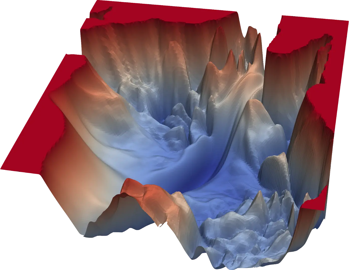
Loss landscape - A 3D surface plot of the loss of ResNet-110-noshot (Li et al., 2017)
Loss Functions
The loss function (also known as the cost function, objective function or criterion) computes the extent to which the neural network’s ouput differs from the expected output. Loss functions depend on the architecture of a neural network and its expected output, which are task-dependent. The value calculated by the loss function is referred to as loss.
Mean Squared Error
The mean squared error (MSE) is the average of the squared differences between the predicted and expected values:
\[MSE(y, \hat{y}) = \frac{1}{n}\sum\limits_{i=1}^n (y_i - \hat{y}_i)^2\]where \(n\) is the number of data points, \(y\) are the expected values, and \(\hat{y}\) are the predicted values.
As a loss function, MSE is used primarily in regression problems where a real-value quantity must be predicted. It is sometimes referred to as the quadratic loss function.
def mse(y, pred):
    """Mean squared error loss"""
    return ((y - pred)**2).mean(axis=None)

mse(pred=np.array([[2.5, 0.0, 2, 8]]), y=np.array([[3, -0.5, 2, 7]]))
0.375
Cross-Entropy (Log Loss)
A common task in deep learning is classification, where a set of inputs has to be matched to a set of class labels. Classification can be modelled as predicting the probability that a given input belongs to a certain class.
Cross-entropy can be used to calculate the difference between an expected and predicted probability distributions. Each predicted probability is compared with its expected probability and scored logarithmically. Small differences therefore lead to small scores and large differences to large scores.
\[CE(y, \hat{y}) = -\sum_{i} y_i log(\hat{y}_i)\]def cross_entropy(y, pred):
"""Cross-entropy loss"""
pred = np.maximum(1e-15, np.minimum(1 - 1e-15, pred))
return -np.sum(y * np.log(pred + 1e-15)) / y.shape[0]
# Note that `y` and `pred` must have a batch dimension, since we
# divide the total loss by the number of sample in the batch.
y = np.array([[1, 0, 0]])
predicted = np.array([[0.6, 0.1, 0.3]])
cross_entropy(y, predicted)
0.5108256237659891
# A perfect prediction has a score of 0.0
cross_entropy(y, y)
-0.0
# On batches, the mean cross-entropy loss is returned
y = np.array([
    [1, 0, 0],
    [1, 0, 0]
])
predicted = np.array([
    [0.6, 0.1, 0.3],
    [0.6, 0.1, 0.3]
])
cross_entropy(y, predicted)
0.5108256237659891
Beyond mean squared error and cross entropy loss, other loss function include the hinge loss, the huber loss, the Kullback-Leibler (KL) divergence and the mean absolute error.
The Backpropagation Algorithm
Backwards propagation of errors, or backpropagation, is a method for calculating the gradient of the loss function \(\nabla L\) with respect to the network’s weights and biases \(w, b\) for a given set of inputs. The gradient \(\nabla L\) is therefore given by:
\[\nabla L = \begin{bmatrix} \nabla_w L, \nabla_b L \end{bmatrix}\]where \(\nabla_w L\) denotes the Jacobians for all weight matrices in the network and \(\nabla_b L\) the vectors for all biases.
\[\nabla_w L = \begin{bmatrix} \dfrac{\partial L}{\partial w^0_{jk}}, \dfrac{\partial L}{\partial w^1_{jk}}, \dots, \dfrac{\partial L}{\partial w^l_{jk}} \\ \end{bmatrix}\] \[\nabla_b L = \begin{bmatrix} \dfrac{\partial L}{\partial b^0_j}, \dfrac{\partial L}{\partial b^1_j}, \dots, \dfrac{\partial L}{\partial b^l_j} \\ \end{bmatrix}\]Given the loss \(L\) for a set of inputs, backpropagation consists in recursively computing the partial derivative for all variables in the computational graph by application of the chain rule.
Chain rule reminder: Let \(x\) be a real number and \(f\) and \(g\) two functions mapping from a real number to a real number. If \(z = g(x)\) and \(y = f(g(x)) = f(z)\), the derivative between \(y\) and \(x\) is
\[\frac{\partial y}{\partial x} = \frac{\partial y}{\partial z}\frac{\partial z}{\partial x}\]For example, the function \(y = σ(w⋅x + b)\) can be expressed as the following computational graph.

The partial derivative between the loss \(L\) and the weights \(w\) is given by:
\[\nabla_w L = \frac{\partial L}{\partial \hat{y}} \frac{\partial \hat{y}}{\partial z} \frac{\partial z}{\partial u} \frac{\partial u}{\partial w}\]We can similarly relate the loss \(L\) to the bias \(b\):
\[\nabla_b L = \frac{\partial L}{\partial \hat{y}} \frac{\partial \hat{y}}{\partial z} \frac{\partial z}{\partial b}\]By using the chain rule, we can compute these partial derivatives by calculating the derivatives for all operations. Loss functions are multivariate, but since the expected output \(y\) is fixed, we only need the partial derivative with respect to the real output \(\hat{y}\). In this example, we use the mean squared error loss function. The sigmoid function, like all activation functions, has one variable and therefore only one derivative.
\[L = MSE(y, \hat{y}) \qquad\rightarrow \qquad \frac{\partial L}{\partial \hat{y}} = -2(y - \hat{y})\] \[\sigma(z) = \dfrac{1}{1 + e^{-z}} \qquad\rightarrow \qquad \dfrac{d\sigma}{dz} = \sigma(z)(1-\sigma(z))\] \[f(b, u) = b + u \qquad\rightarrow \qquad \frac{\partial f}{\partial b} = 1 \qquad \frac{\partial f}{\partial u} = 1\]For the matrix multiplication operation, the partial derivative is the transpose of the variable held constant.
\[f(w, x) = wx \qquad\rightarrow \qquad \frac{\partial f}{\partial w} = x^T \qquad \frac{\partial f}{\partial x} = w^T\]Given these partial derivatives, we can express \(\nabla_w L\) and \(\nabla_b L\) as follows:
\[\nabla_w L = -2(y - \hat{y})\cdot (\sigma(z)(1-\sigma(z)) )\cdot 1 \cdot x^T\] \[\nabla_b L = -2(y - \hat{y})\cdot (\sigma(z)(1-\sigma(z))) \cdot 1\]Backpropagation consists in computing these expressions progressively as we move backwards though the network. This operation is denoted as the backward pass.
Note: the principles outlined above apply to tensors of any rank (i.e. vectors and matrices). However, when implementing backpropagation, it is important to pay attention to the dimensionality of the tensors and choose whether to do an element-wise multiplication or a matrix multiplication. In the implementation below, \(\partial L / \partial \hat{y}\) and \(\partial \hat{y} / \partial z\) are both tensors of rank 1 so that \((\partial L / \partial \hat{y}) \cdot (\partial \hat{y} / \partial z)\) is an element-wise multiplication (Hadamard product) of both tensors. On the other hand, \((\partial z / \partial u) \cdot (\partial u / \partial w)\) is a matrix multiplication.
x = np.array([[1.4, 0.62, 0.21]])
w = np.array([[0.18], [0.24], [-0.2]])
b = np.array([[0.5]])
y = np.array([[1]])

# Forward pass
z = x @ w + b
pred = sigmoid(z)

# Backward pass
dL_dpred = -2 * (y-pred)
dL_dz = dL_dpred * sigmoid(z, derivative=True)
grad_b = dL_dz
grad_w = x.T @ dL_dz

print(f"Gradient of L over w: {grad_w}")
print(f"Gradient of L over b: {grad_b}")
Gradient of L over w: [[-0.17417494] [-0.07713462] [-0.02612624]] Gradient of L over b: [[-0.12441067]]
Intermediate values from the forward pass such as \(z\) are cached to be reused for the backward pass.
We can verify the result of our backward pass numerically using the finite difference method. Below, we calculate \(\nabla_{w_1}L\).
def forward(w, b, x, y):
    """Forward pass"""
    z = x @ w + b
    pred = sigmoid(z)
    loss = mse(y, pred)
    return loss

(forward(np.array([0.1801, 0.24, -0.2]), b, x, y) - forward(np.array([0.1799, 0.24, -0.2]), b, x, y)) / 0.0002
-0.17417493743975
On deeper computational graphs, we would continue backpropagating the loss as follows:
dL_dx = dL_dz @ w.T
# dL_dz0 = dL_dx * sigmoid(z0, derivative=True)
# grad_b0 = dL_dz0
# grad_w0 = x0.T @ dL_dz0
# ...
With batches, we can take the mean of the gradients over all samples in the batch to calculate the gradient over the batch. The matrix multiplication x.T @ dL_dz already sums the gradients along the batch dimension, so we only need to divide its result by the number of samples in the batch.
grad_b = np.mean(dL_dz, axis=0, keepdims=True)
grad_w = x.T @ dL_dz / x.shape[0]
The partial derivatives in backpropagation are nowadays seldom defined and implemented by hand. Modern deep learning frameworks use automatic differentation (also called autodiff or autograd) to determine the derivative of a function. Automatic differentiation is a more general technique than backpropagation, but similarly uses the chain rule to calculate the derivative of a function by deconstructing it into elemental operations with known derivatives. Deep learning libraries that use a define-and-run approach pre-define common functions and their derivatives and allow users to build a model by combining them into a static computational graph. Another approach, known as define-by-run, is to dynamically build a computational graph and calculate its derivatives during execution. With this approach, a user typically builds a model by writing the forward pass.
Optimizers
Optimization consists in maximizing or minimizing a real function by systematically altering its input and computing the value of the function. For some function \(f: \mathbb{R} \rightarrow \mathbb{R}\), we denote the value of the argument \(x\) that minimizes \(f\) as follows:
\[\arg \min_{x \in \mathbb{R}} f(x)\]Gradient descent is an iterative first-order optimization algorithm. Given a multivariate function \(f: \mathbb{R}^m \rightarrow \mathbb{R}\), it consists in iteratively decreasing \(f\) by moving in the direction of the negative gradient \(-\nabla_x f(x)\). For each iteration \(n\), we find the new value \(x_{n+1}\) in the sequence \((x_{n})\):
\[x_{n+1} = x - \eta \nabla_x f(x)\]in the hope that the sequence eventually converges to a local minimum. The learning rate \(\eta \in \mathbb{R}_+\) determines the size of the steps taken at each iteration. The learning rate is a crucial parameter. A high learning rate will make larger steps and might converge faster, but risks being unable to settle near the local optimum. A low learning rate will make smaller, more careful steps, but will need more iterations to converge. On non-convex surfaces, small learning rates are also more likely to get stuck in bad local optimums.
In deep learning, the objective is to find the best parameters \(\theta\) that minimize the loss function \(J\) based on a training set comprised of the inputs \(x\) and corresponding labels \(y\).
\[\arg \min_{\theta} J(\theta; x, y)\]The conventional approach is to solve this optimization problem using a variant of gradient descent.
Throughout this section, we graph the optimizers using test functions for optimization algorithms, which are also known as artificial landscapes. One such function is the McCormick function, defined as:
\[z = f(x, y) = sin(x + y) + (x - y)^2 - 1.5x + 2.5y + 1\]The McCormick function is usually evaluated on the input domain \(x \in [-1.5, 4], y \in [-3, 4]\). The minimum on this domain is \(z_{min} = f(x^*, y^*) = -1.91322\) where \(x^* = -0.54719\) and \(y^* = -1.54719)\). We use a modified version of the McCormick function with a z-intercept of \(3\) instead of \(1\) so that \(z_{min} = 0,08678\).
def mccormick(x, y):
    """McCormick function"""
    return np.sin(x + y) + (x - y)**2 - 1.5*x + 2.5*y + 3
The gradient of the McCormick function can be derived as follows:
\[\nabla_{x, y} f = \begin{bmatrix} \dfrac{\partial f}{\partial x}, \dfrac{\partial f}{\partial y} \end{bmatrix}\]where,
\[\dfrac{\partial f}{\partial x} = cos(x + y) + 2x - 2y -1.5\] \[\dfrac{\partial f}{\partial y} = cos(x + y) + 2y - 2x -2.5\]def grad_mccormick(x, y):
"""Gradient of the McCormick function"""
dx = np.cos(x + y) + 2*x -2*y - 1.5
dy = np.cos(x + y) + 2*y -2*x + 2.5
return np.array([dx, dy])
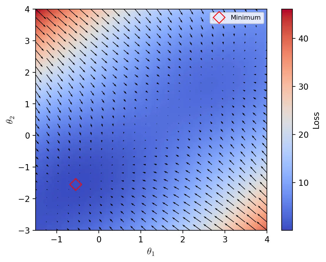
A heatmap of the McCormick function, which is used as an artificial loss landscape. The quivers indicate the direction of the negative gradient.
Batch Gradient Descent
Batch gradient descent, sometimes denoted as vanilla or full-batch gradient descent, uses the gradient of the loss function for all training examples \(\nabla_{\theta}J(\theta; x,y)\), i.e. the true gradient, to update the parameters of the model. Each update consists in adding the product of the learning rate \(\eta\) and the negative gradient \(-\nabla_{\theta}J(\theta; x, y)\) to the parameters \(\theta\).
\[\theta \leftarrow \theta - \eta \cdot \nabla_{\theta}J(\theta; x, y)\]Computing the true gradient for each update is slow and considerably slows down training. For this reason, other optimiziation algorithms that compute the gradient using a fraction of the dataset are usually preferred over batch gradient descent.
def bgd(params: np.ndarray, lr: float, epochs: int):
    """Batch gradient descent"""
    for epoch in range(epochs):
        grad = grad_mccormick(*params)
        params = params - lr * grad
        yield params

start = np.array([-1., 2.75])
bgd_mccormick = list(bgd(start, lr=0.01, epochs=10000))

Stochastic Gradient Descent
Stochastic gradient descent (SGD) uses an approximation of the gradient \(\nabla_{\theta}J(\theta; x, y)\) to optimize \(J\). At each iteration, SGD randomly selects a training sample \(x^{(i)}\) and its corresponding expected value \(y^{(i)}\) to compute a stochastic approximation of the gradient and update the parameters \(\theta\).
\[\theta \leftarrow \theta - \eta \cdot \nabla_{\theta}J(\theta; x^{(i)}, y^{(i)})\]Samples are drawn either by randomly sampling the training data at each iteration, or by shuffling the dataset at each epoch and completing a whole pass through it. In its purest form, SGD uses a sample size of \(1\), but it can be generalized to larger sample sizes (see mini-batch gradient descent).
Stochasticity: Under the Hood
The gradient for all training examples \(\nabla_{\theta}J(\theta; x, y)\) is the mean of the gradients of all training examples \(\nabla_{\theta}J(\theta; x^{(i)}, y^{(i)})\).
\[\nabla_{\theta}J(\theta; x, y) = \frac{1}{n}\sum_{i=1}^n \nabla_{\theta}J(\theta; x^{(i)}, y^{(i)})\]Each training example is unique and its gradient can differ significantly from that of other training examples. For a given parameter \(\theta_j\), the partial derivative \(\partial L / \partial \theta_j\) depends on the random sample of training data. The distribution of the partial derivatives \(\partial L / \partial \theta_j\) of all training examples can therefore be described by a probability density function \(P\):
\[\dfrac{\partial L}{\partial \theta_j} \sim P\]The shape, mean and standard deviation of \(P\) depends on the model architecture, training dataset, and parameter in question. The mean and variance of the partial derivatives for one parameter can thus be drastically different than for another.
SGD randomly samples the probability distributions of gradients and is therefore a stochastic method, i.e. it is well described by a random probability distribution.
Note: the adjectives “random” and “stochastic” can be used interchangeably. “Random” is commonly used to describe a variable while “stochastic” is used to describe a process.
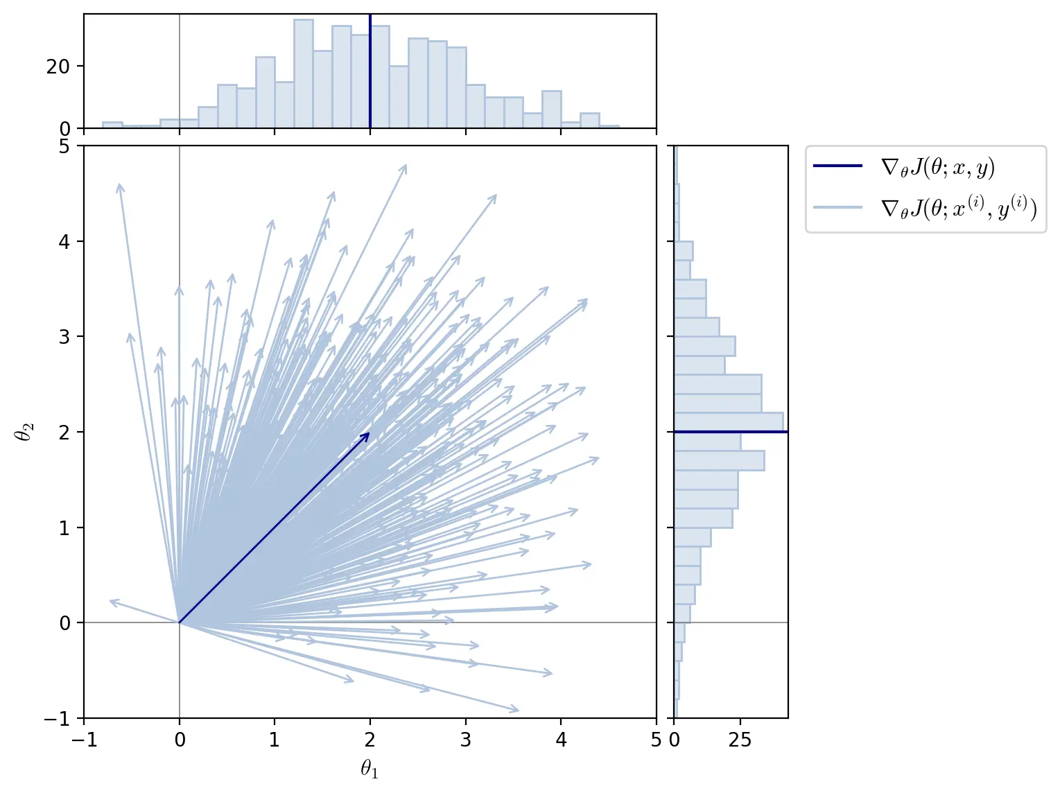
The figure above illustrates a distribution of gradients for two parameters \(\theta_1\) and \(\theta_2\). The mean of all gradients \(\nabla_{\theta}J(\theta; x, y) = [2, 2]\). The gradients of the training examples \(\nabla_{\theta}J(\theta; x^{(i)}, y^{(i)})\) are represented as following a normal distribution with standard deviation of \(1\) on both parameters \(\theta_1\) and \(\theta_2\).
Simulated Stochasticity
The optimization of artificial landscapes such as the McCormick function is inherently different from that of neural networks. Artificial landscapes are optimized with respect to their real variables and their gradients cannot therefore be approximated stochastically. However, to simulate the stochasticity of SGD, we can create an artificial stochastic process that generates approximate gradients.
We assume that the partial derivatives over the parameters \(\theta_1\) and \(\theta_2\) follow normal distributions with standard deviation of 16 and 4, respectively. These distributions are kept constant for all parameter values (this is not very realistic, but is good enough for our purpose). The key variables of our simulation are the dataset and batch size, which determine the expected accuracy of the approximated gradient. The dataset size is set to 40.
Based on the real gradient of the McCormick function, we draw 40 samples for each parameter according to the assumptions outlined above. These samples represent the gradients of all instances in the fictional dataset. The gradients are then normalized so that their mean corresponds to the real gradient. Finally, the approximation of the gradient is calculated by sampling a batch of gradients and finding its mean.
DATASET_SIZE = 2000

def simulate_grad(params, batch):
    """Synthetic simulation of the gradient"""
    # Calculate the real gradient
    grad = grad_mccormick(*params)
    # Generate a distribution of partial derivatives of x with standard deviation of 16
    distx = np.random.normal(grad[0], 16, size=(DATASET_SIZE, 1))
    distx += grad[0] - distx.sum() / DATASET_SIZE
    # Generate a distribution of partial derivatives of y with standard deviation of 4
    disty = np.random.normal(grad[1], 4, size=(DATASET_SIZE, 1))
    disty += grad[1] - disty.sum() / DATASET_SIZE
    grads = np.concatenate((distx, disty), axis=1)
    # Sample a mini-batch and find its mean gradient
    batch_size = len(batch)
    idx = np.random.choice(grads.shape[0], batch_size, replace=False)
    grads = grads[idx, :]
    return grads.sum(axis=0) / batch_size
Based on this simulated gradient approximation, we can plot the path of SGD. The dataset is usually shuffled at each epoch, but this step is omitted here.
def sgd(data, params: np.ndarray, lr: float, epochs: int):
    """Stochastic Gradient Descent"""
    for epoch in range(epochs):
        for instance in data:
            grad = simulate_grad(params, [instance])
            params = params - lr * grad
            yield params

data = np.linspace(0, 1, DATASET_SIZE)
sgd_mccormick = list(sgd(data, start, lr=0.001, epochs=2))
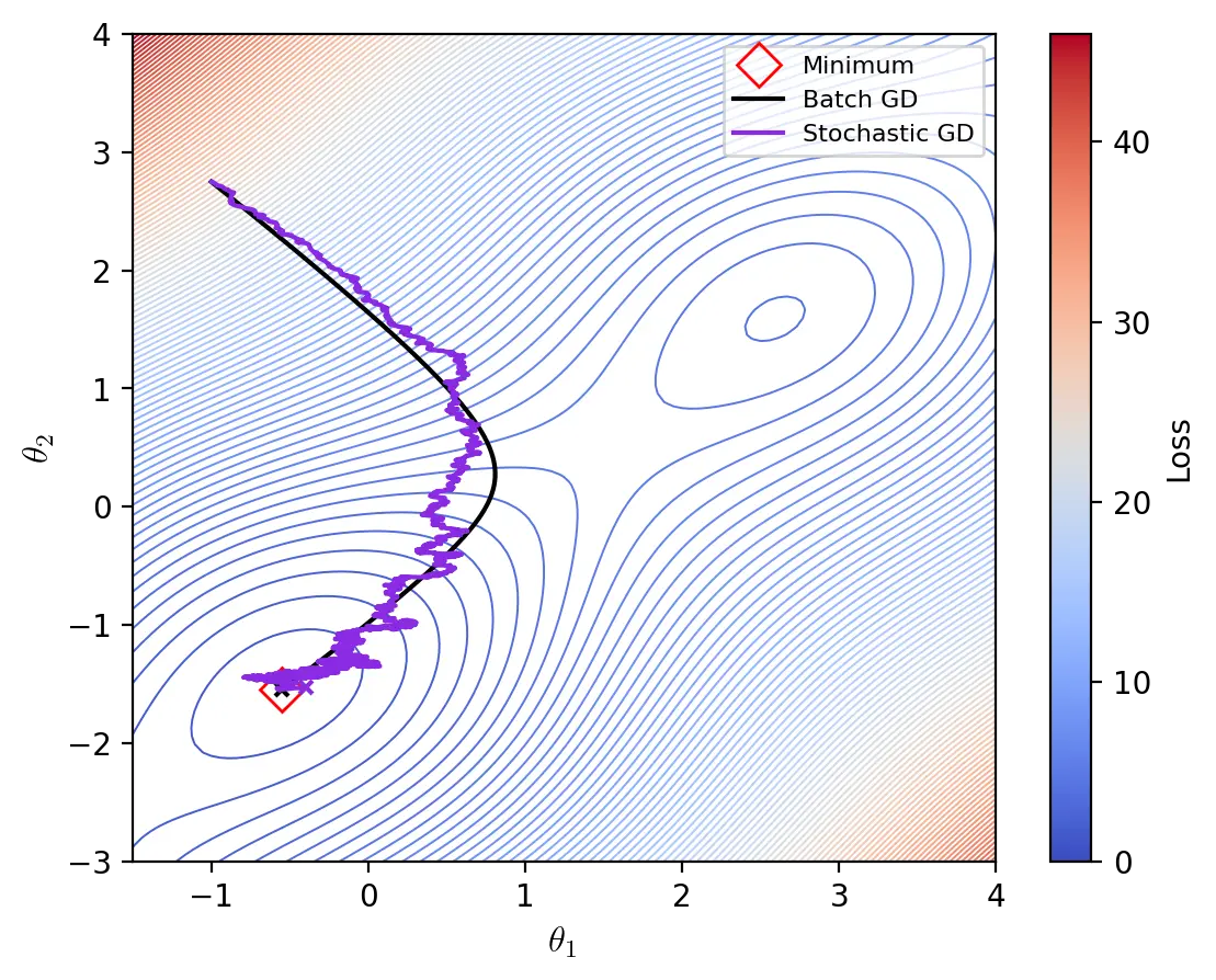
The primary advantage of SGD over batch gradient descent is that it is less computationally expensive and therefore converges faster. However, by computing only an approximation of the true gradient, SGD makes a tradeoff between speed and precision of convergence. While batch gradient descent has small gradients near minima, SGD can struggle to settle near minima due to its high stochasticity.
Mini-batch Gradient Descent
Mini-batch gradient descent is a generalization of batch and stochastic gradient to any sample size. Every update is performed with a batch of \(n\) training examples:
\[\theta \leftarrow \theta - \eta \cdot \nabla_{\theta}J(\theta; x^{(i:i+n)}, y^{(i:i+n)})\]The advantage of mini-batch gradient descent is that using a batch size larger than \(1\) improves the accuracy of the approximated gradient. Moreover, thanks to highly-optimized linear algebra libraries, computing the gradient of mini-batches that fit into memory is often only marginally slower than computing it for a single training example. However, the accuracy of the approximated gradient, as measured by the standard error of the mean, increases less than linearly. The standard error of the mean \(\sigma_{\bar{x}}\) is given by:
\[\sigma_{\bar{x}} = \frac{\sigma}{\sqrt{n}}\]where \(\sigma\) is the true standard deviation of the distribution and \(n\) is the number of samples drawn. The factor \(1 / \sqrt{n}\) indicates that reducing the standard error of the mean requires exponentially more samples. Beyond a certain size, large batches have therefore diminishing returns. Memory and IO bandwidth limit vectorization and it becomes preferable to update the parameters more frequently rather than calculate more accurate gradients.
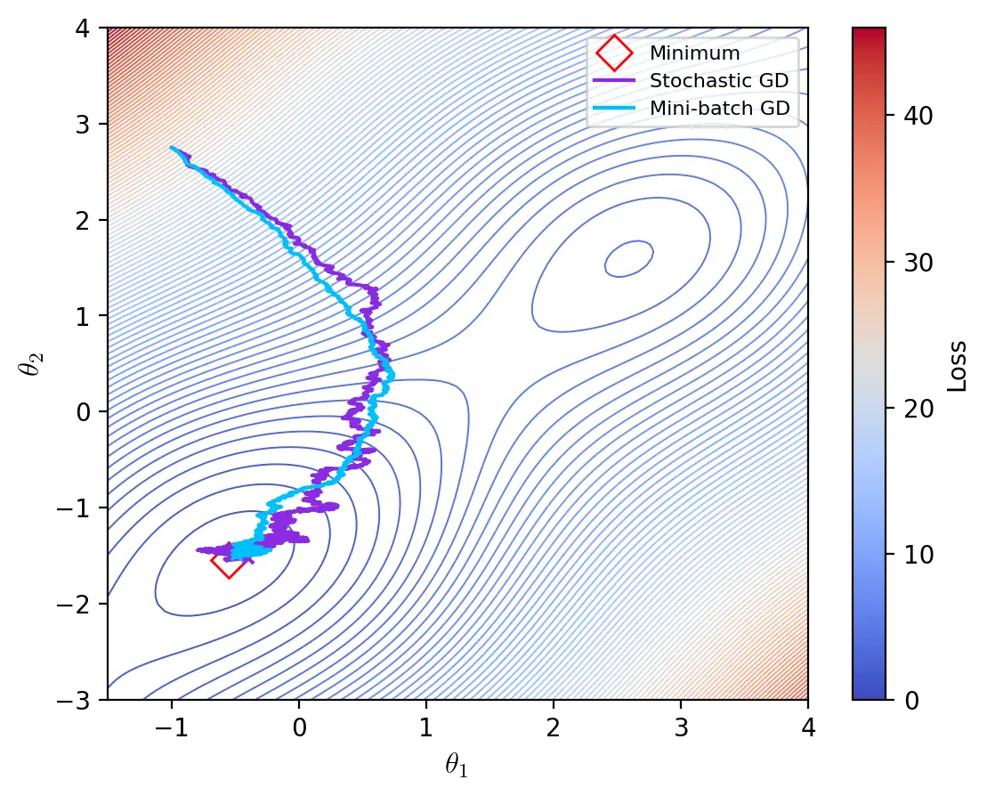
Note that the number of epochs is not indicative of the speed in wall-clock time of an optimizer. The number of epochs, together with the batch size, merely indicates the number of updates the optimizers performs until it converges. To assess the speed of an optimizer we would need to analyse the time complexity of the gradient calculation and parameter update, or run an experiment.
Momentum
Momentum calculates an exponentially decaying moving average of past gradients to update the parameters. A variable \(v\) represents this decaying moving average as the velocity of the gradients. For each update \(t\), the momentum algorithm adds a fraction \(\gamma \in [0,1)\) of the previous velocity \(v_{t-1}\) to the current update vector:
\[v_t = \gamma v_{t-1} + \eta\nabla_{\theta}J(\theta)\] \[\theta \leftarrow \theta - v_t\]The momentum term \(\gamma\) determines how quickly the velocity decays. A typical value for \(\gamma\) is \(0.9\).
def momentum(params: np.ndarray, lr: float, gamma:float, epochs: int, batch_size):
    """Momentum optimizer"""
    velocity = np.zeros(params.shape)
    for epoch in range(epochs):
        for i in range(0, len(data), batch_size):
            batch = data[i:i+batch_size]
            grad = simulate_grad(params, batch)
            update = gamma * velocity + lr * grad
            params = params - update
            velocity = update
            yield params

path = list(momentum(start, lr=0.00005, gamma=0.98, epochs=10, batch_size=4))
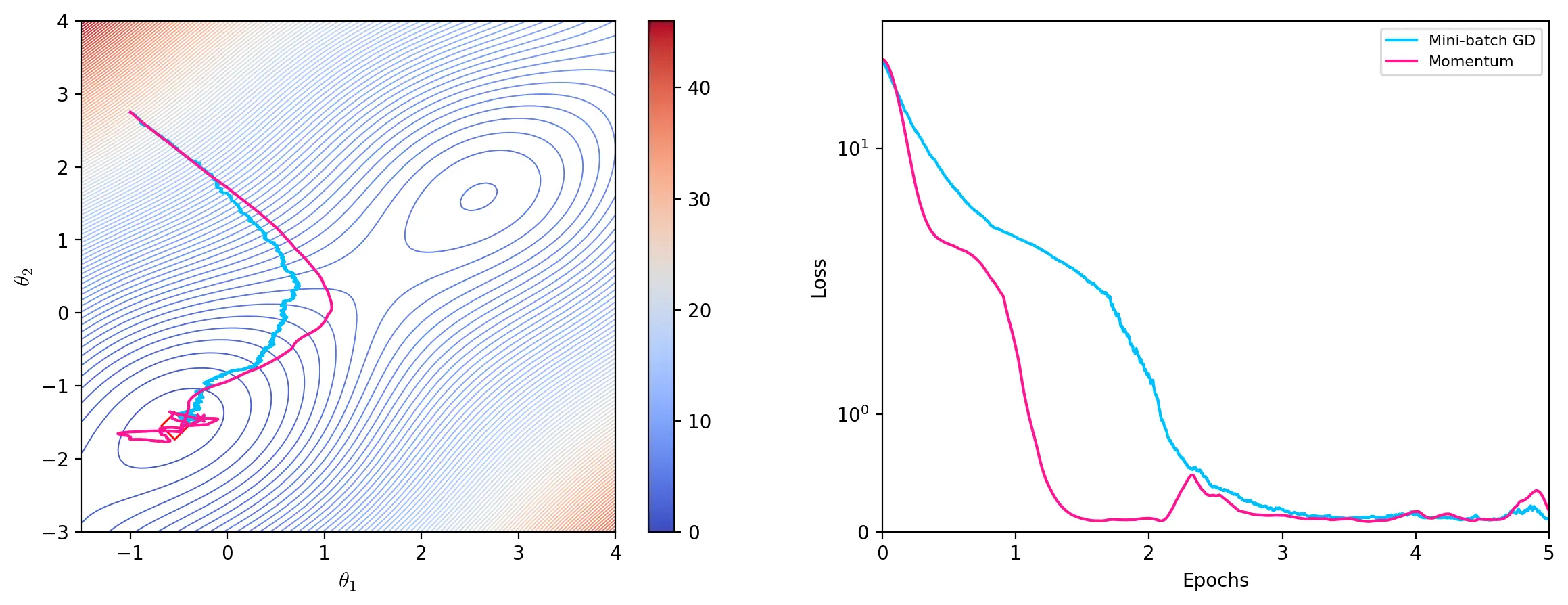
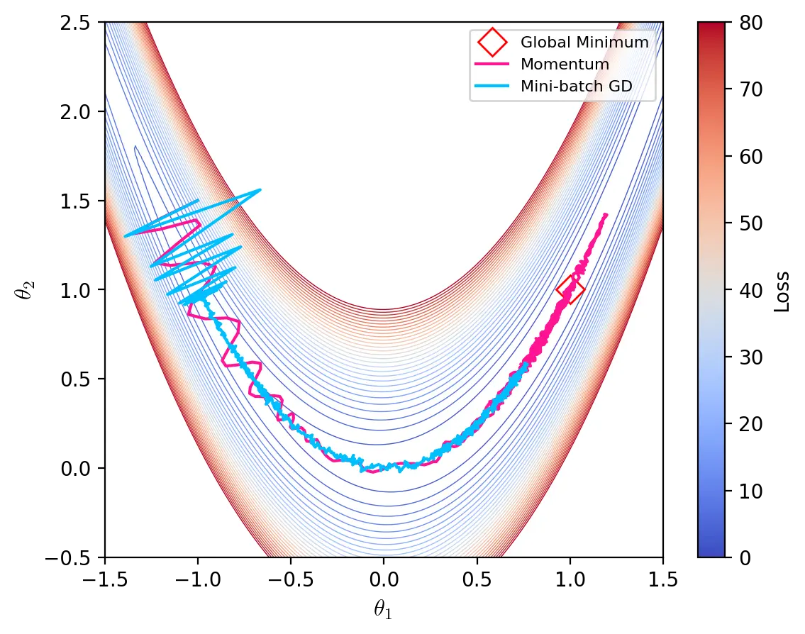
The graph below illustrates some of the characteristics of momentum and mini-batch gradient descent on the artificial landscape generated by the Rosenbrock function. Momentum is able to navigate through the ravine and settle near the global minimum while mini-batch gradient descent oscillates at the start and struggles to advance through the bottom of the ravine where gradients are small.
Adagrad
Adagrad (Duchi et al., 2011), short for Adaptive Gradient Algorithm, adapts the learning rate individually to all parameters during training. For each update, Adagrad scales the learning rate for each parameter by dividing it by the square root of the outer product matrix \(G_t\), given by:
\[G_t = \sum^t_{\tau=1} g_{\tau}g_{\tau}^\top\]where \(g_{\tau}\) denotes the gradient at iteration \(\tau\). Since calculating the square root of \(G_t\) is computationally impractical, we update the parameters using its diagonal, \(diag(G_t)\), which is effectively the sum of the historical squared gradients of all parameters (ibid, p. 2122).
g = np.array([[-1., 2.75]])
(np.diagonal(g * g.T) == g**2).all()
True
The update vector is then the element-wise multiplication (Hadamard product) of the learning rates and the gradient:
\[\theta \leftarrow \theta - \frac{\eta}{\epsilon + \sqrt{diag(G_t)}} \odot g_t\]where \(\epsilon\) is a smoothing term used to avoid division by zero.
def adagrad(data, params: np.ndarray, lr: float, epochs, batch_size: int, eps=1e-8):
    """Adagrad optimizer"""
    Gt = np.zeros(params.shape)
    for epoch in range(epochs):
        for i in range(0, len(data), batch_size):
            batch = data[i:i+batch_size]
            grad = simulate_grad(params, batch)
            Gt += grad**2
            update = lr / np.sqrt(Gt + eps) * grad
            params = params - update
            yield params

path = list(adagrad(data, start, lr=0.15, epochs=10, batch_size=4))
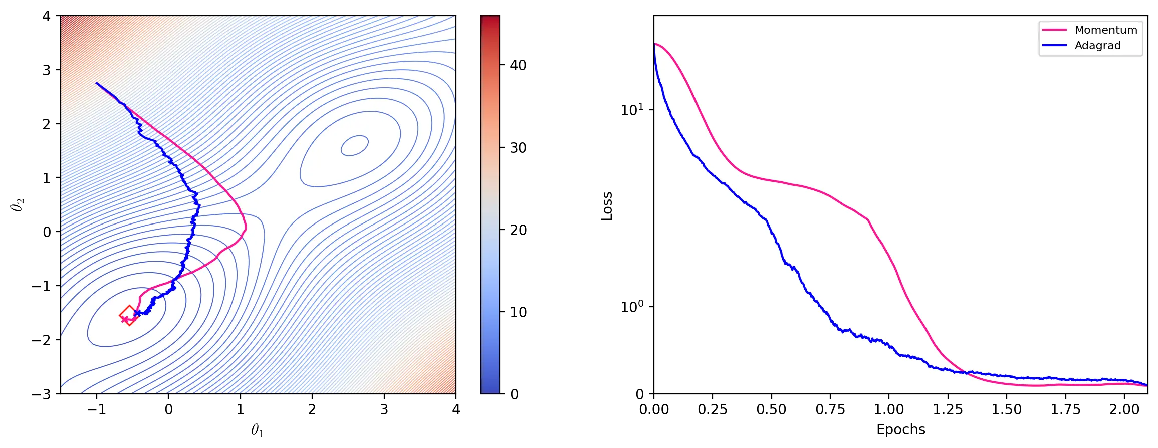
Like other optimizers with adaptive learning rates, Adagrad is able to finely adjust parameters to which the model is highly sensitive. However, the accumulation of past squared gradients monotonously decreases the learning rate, which can become infinitesimally small. Such aggressive decreases of the learning rate can sometimes prevent or slow down convergence.
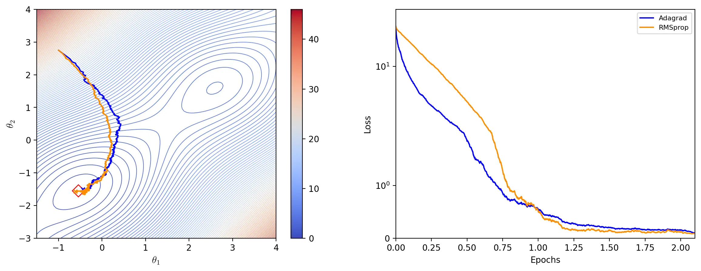
RMSprop
RMSprop (Hinton, 2012) seeks to address the shortfalls of Adagrad by using an exponentially decaying average of past squared gradients to adapt the learning rate. The average \(E[g^2]_t\) for each update \(t\) is given by:
\[E[g^2]_t = \gamma E[g^2]_{t-1} + (1 - \gamma)g^2_t\]where \(g_t\) is the current gradient and \(\gamma \in [0, 1)\) is the decay factor. The update rule is similar to that of Adagrad:
\[\theta \leftarrow \theta - \frac{\eta}{\epsilon + \sqrt{E[g^2]_t}} \odot g_t\]Hinton (2012) recommends setting \(\gamma\) to \(0.9\) and the learning rate to \(0.001\) (slide 29).
def rmsprop(data, params: np.ndarray, lr: float, epochs: int, gamma:float, batch_size: int, eps=1e-8):
    """RMSprop optimizer"""
    average = np.zeros(params.shape)
    for epoch in range(epochs):
        for i in range(0, len(data), batch_size):
            batch = data[i:i+batch_size]
            grad = simulate_grad(params, batch)
            average = gamma * average + (1 - gamma) * grad**2
            update = lr / np.sqrt(average + eps) * grad
            params = params - update
            yield params

path = list(rmsprop(data, start, lr=0.01, epochs=10, gamma=0.9, batch_size=4))
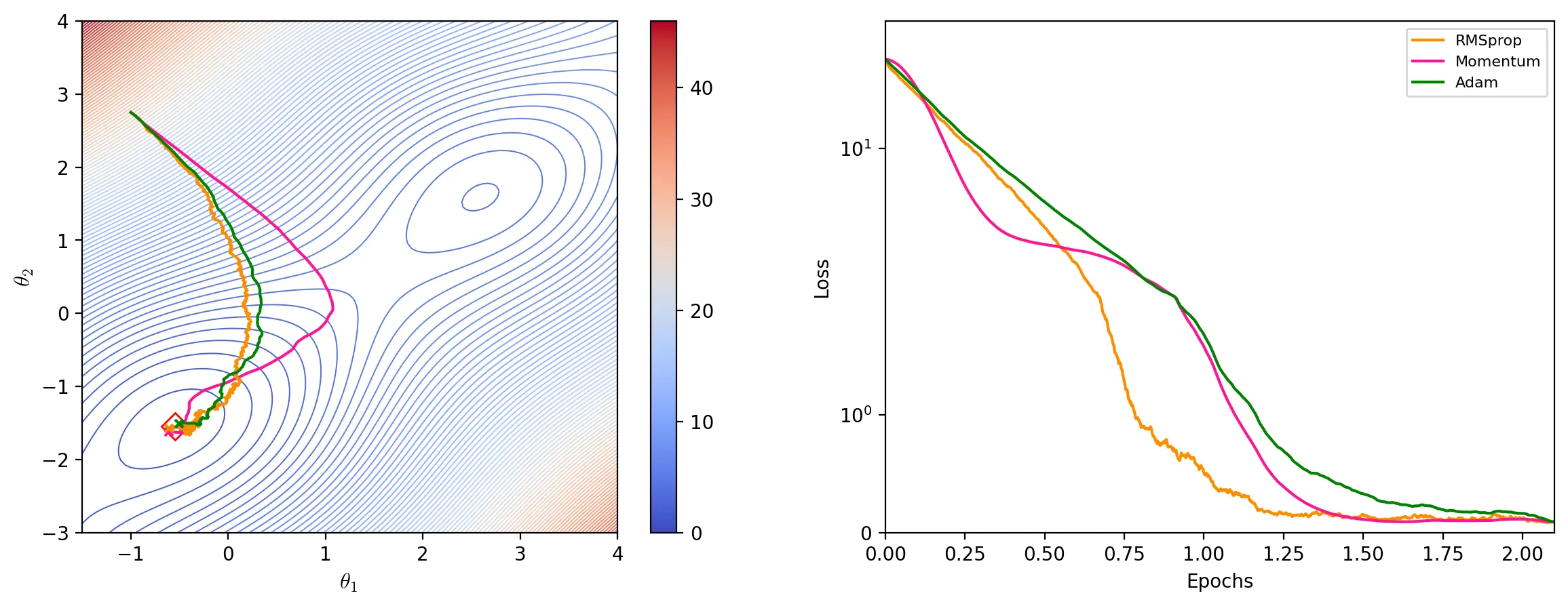
Adam
Adam (Kingma and Ba, 2015), which stands for Adaptive Moment Estimation, is another adaptive learning rate optimizer. Adam uses estimates of the mean (1st moment) and uncentered variance (2nd moment) of the gradient to update the parameters. The estimate of the mean is given by the exponential moving average of the gradient \(m_t\):
\[m_t = \beta_1 m_{t - 1} + (1 - \beta_1)g_t\]The estimate of the variance is given, like for RMSprop, by the exponential moving average of the squared gradient \(v_t\):
\[v_t = \beta_2 v_{t - 1} + (1 - \beta_2)g_t^2\]The moving averages are initialized as vectors of 0’s and, particularly during the first steps, are therefore biased towards zero. Adam therefore calculates the bias-corrected estimates \(\hat{m_t}\) and \(\hat{v_t}\):
\[\hat{m_t} = \frac{m_t}{1 - \beta_1^t}\] \[\hat{v_t} = \frac{v_t}{1 - \beta_2^t}\]\(\beta_1^t\) and \(\beta_2^t\) denote \(\beta_1\) and \(\beta_2\) to the power of \(t\). Updating the parameters consists in adapting the learning rate to the parameters based on \(v_t\) and multiplying these individual learning rates with \(\hat{m_t}\):
\[\theta \leftarrow \theta - \frac{\eta}{\epsilon + \sqrt{\hat{v_t}}} \odot \hat{m_t}\]Kingma and Ba (2015) suggest using \(\beta_1 = 0.9\) and \(\beta_2 = 0.999\) as defaults.
def adam(data, params: np.ndarray, lr: float, epochs, b1, b2, batch_size: int, eps=1e-8):
    """Adam optimizer"""
    t = 0
    m = np.zeros(params.shape)
    v = np.zeros(params.shape)
    for epoch in range(epochs):
        for i in range(0, len(data), batch_size):
            t += 1
            batch = data[i:i+batch_size]
            grad = simulate_grad(params, batch)
            m = b1 * m + (1 - b1) * grad
            v = b2 * v + (1 - b2) * grad**2
            m_hat = m / (1 - b1**t)
            v_hat = v / (1 - b2**t)
            params = params - (lr / (np.sqrt(v_hat) + eps) * m_hat)
            yield params

path = list(adam(data, start, lr=0.01, epochs=10, b1=0.9, b2=0.999, batch_size=4))
An animation of the different gradient descent algorithms is available here.
Hazards
Dying ReLU neurons
ReLU neurons output zero if their weighted sum is negative (i.e. when they have negative weights, negative inputs or a large negative bias). While this property can be beneficial in the form of sparsity, it can become problematic if a neuron consistently outputs zero for any input values. Since \(RELU’(z) = 0\) when \(z <= 0\), the parameters are not updated and the neuron dies.
Mini-batch stochastic gradient descent generates new batches at each iteration and, as long as not all inputs lead to a negative weighted sum, can prevent a neuron from becoming completely inactive. However, a high learning-rate can also lead to consistently negative weighted sums by updating the weights to high negative values. A lower learning rate or the use of an alternative activation function such as Leaky ReLU can mitigate this issue.
Vanishing gradients
Gradients can diminish drastically when they are backpropagated through a deep neural network during training. By the time the error reaches the first layers, the gradient can become so small that it is “difficult to know [in] which direction the parameters should move to improve the cost function” (Goodfellow et al, 2016, p. 290). Vanishing gradients can slow down and even prevent convergence. This issue is particularly salient in Recurrent Neural Networks (RNNs), which have a high number of steps, or in networks using the sigmoid/tanh activation functions. Alleviations include paying special attention to the weight initialization scheme, or using an alternative activation function.
Initialization
[…] training deep models is a sufficiently difficult task that most algorithms are strongly affected by the choice of initialization. The initial point can determine whether the algorithm converges at all, with some initial points being so unstable that the algorithm encounters numerical difficulties and fails altogether.
(Goodfellow et al., 2016, p. 301)
A key function of initialization is to break the symmetry between different neurons. If all parameters in a given dense layer were initialized with the same constant, they would all compute the same ouputs and receive the same updates. Random initialization breaks this symmetry and creates asymmetries that can be tweaked through backpropagation and SGD to train the neural network.
Typically, only the weights are initialized randomly while the biases are set to a heuristically chosen constant.
A simple method of weight intialization is to sample values from a Gaussian probability distribution with mean 0 and a standard deviation of 1.
neurons = 256
inputs = 512

weights = np.random.randn(inputs, neurons)
print(f"Minimum: {weights.min():.4f}   Maximum: {weights.max():.4f}")
print(f"Mean:    {weights.mean():.4f}   SD: {weights.std():.4f}")
Minimum: -4.4978 Maximum: 4.1724 Mean: 0.0018 SD: 1.0009
Glorot and Bengio (2010) suggest initializing a neuron’s weights using a uniform probability distribution with mean 0.0 and a range that depends on the number of inputs \(m\) and number of outputs \(n\) of the layer.
\[W_{ij} \sim\ U\begin{pmatrix}-\sqrt{\frac{6}{m+n}},\sqrt{\frac{6}{m+n}}\end{pmatrix}\]This method, known as Xavier initialization, maintains the variance of activations and backpropagated errors thoughout the network. Neurons with a sigmoid or tanh activation function are therefore usually initialized with this method to mitigate the issue of vanishing gradients.
def xavier(inputs, neurons):
    """Xavier initialization"""
    limit = np.sqrt(6 / (inputs+neurons))
    weights = np.random.uniform(low=-limit, high=limit, size=(inputs, neurons))
    return weights

weights = xavier(512, 256)

print(f"Minimum: {weights.min():.4f}   Maximum: {weights.max():.4f}")
print(f"Mean:    {weights.mean():.4f}   SD: {weights.std():.4f}")
Minimum: -0.0884 Maximum: 0.0884 Mean: 0.0002 SD: 0.0511
The larger the number of input and neurons in a layer, the smaller the range of weights.
He et al. (2015) propose a strategy tailored to networks using the ReLU activation function that, similarly to Xavier initialization, would maintain a stable activation variance throughout the network. Weights are initialized using a Gaussian probability distribution with a mean of 0.0 and a standard deviation of \(\sqrt \frac{2}{n}\) where \(n\) is the number of inputs to the neuron, while biases are initialized to zero. This method is now known as He initialization.
def he(inputs, neurons):
    """He initialization"""
    return np.random.randn(inputs, neurons) * np.sqrt(2.0 / inputs)

weights = he(512, 256)

print(f"Minimum: {weights.min():.4f}   Maximum: {weights.max():.4f}")
print(f"Mean:    {weights.mean():.4f}   SD: {weights.std():.4f}")
Minimum: -0.2562 Maximum: 0.2892 Mean: 0.0001 SD: 0.0625
Overfitting/Underfitting
The central challenge in machine learning is to perform well on new, previously unseen inputs. Machine learning models are optimized on a known set of data, but their merit depends on their ability to make reliable predictions on cases they were not trained on. This ability is called generalization.
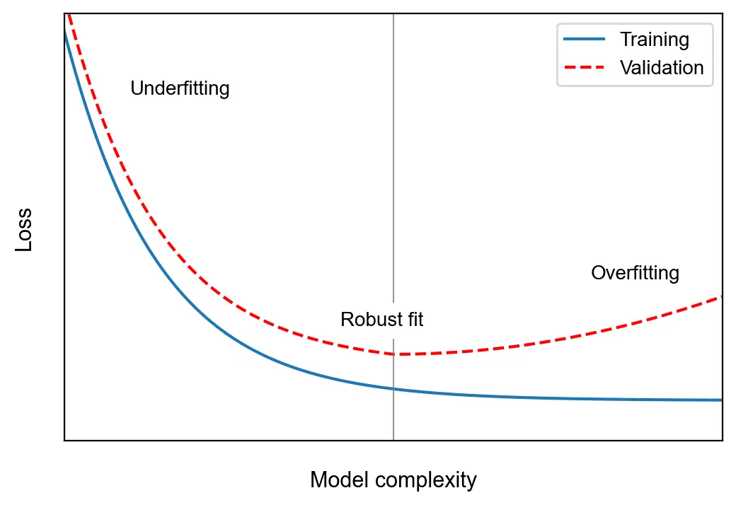
Underfitting occurs when a model is unable to perform well on the training data. Overfitting occurs when it performs well on the training data, but does not generalize well. The reason behind this is that the model learns specific characteristics of the training data that are not general features. Specifically, the model’s parameters become too adapted to the noise in the data and fail to capture its essential features. Overfitting can be addressed by regularizing the model.
Regularization
“Regularization is any modification we make to a learning algorithm that is intended to reduce its generalization error but not its training error” (Goodfellow et al, 2016, p. 120).
Limiting the representative capacity of the network and increasing noise are core strategies that underpin many regularization techniques. The capacity of a model can be limited by decreasing its size or by regularizing its weights. Noise can be injected at the input level through dataset augmentation, at the output level through label smoothing, or at the neuron level through dropout.
Network size
The simplest regularization method is to reduce the size of the model (i.e. lower the total number of neurons). Reducing its size limits the capacity of the model and thus forces it to learn simpler representations. Unfortunately, it is difficult to determine the right network size. In practice, the best model is therefore oftentimes “a large model that has been regularized appropriately” (ibid, p. 229).
Weight regularization
Large weights place a strong emphasis on a few features and lead to high gradients. Weight regularization constrains model complexity by forcing the weights to take on smaller values such that the distribution of weights values becomes more regular. This is achieved by adding to the loss function of the model a penalty associated with having large weights (Chollet, 2021, p. 146). The regularized loss \(L_{reg}\) is given by:
\[L_{reg} = L + \lambda \Omega\]where \(L\) is the unregularized loss, and \(\Omega(\theta)\) is the regularization penalty (\(L^1\) or \(L^2\)). \(\lambda\) > 0 is a hyperparameter that indicates the strength of the preference for smaller weights. Minimizing a loss with weight regularization compels the model to choose weights that “make a tradeoff between fitting the training data and being small” (Goodfellow et al., 2016, p. 119).
\(L^p\) spaces reminder: The \(p\)-norm or \(L^p\)-norm of a vector \(x\) is defined by
\[{\lVert x \rVert}_p = ({\lvert x_1 \rvert}^p + {\lvert x_2 \rvert}^p + ... + {\lvert x_n \rvert}^p)^\frac{1}{p}\]for a real number \(p ≥ 1\).
\(L^1\) regularization
With \(L^1\) regularization, the added penalty is given by the \(L^1\) norm:
\[\Omega = {\left\lVert w \right\rVert}_1 = \sum_i{\lvert w_i \rvert}\]The penalty is therefore proportional to the absolute value of the weight coefficients.
def l1_reg(w: np.ndarray):
    """L1 regularization"""
    return np.sum(np.absolute(w), axis=0)

# Small weights -> small penalty
w = np.array([[-0.15], [0.2], [-0.12], [0.04]])
l1_reg(w)
array([0.51])
# Large weights -> large penalty
w = np.array([[-1.5], [2], [-1.2], [0.4]])
l1_reg(w)
array([5.1])
# Alternative implementation using Numpy's buit-in `norm()` function
np.linalg.norm(w, ord=1, axis=0)
array([5.1])
\(L^2\) regularization
With \(L^2\) regularization (also known as weight decay in deep learning and as ridge regression or Tikhonov regularization in other fields of science) the added penalty is given by the squared \(L^2\) norm:
\[\Omega = {\left\lVert w \right\rVert}_2^2 = w^Tw\]and is therefore proportional to the square of the value of the weight coefficients.
def l2_reg(w: np.ndarray):
    """L2 regularization"""
    return np.sum(w**2, axis=0)

# Small weights -> small penalty
w = np.array([[-0.15], [0.2], [-0.12], [0.04]])
l2_reg(w)
array([0.0785])
# Large weights -> large penalty
w = np.array([[-1.5], [2], [-1.2], [0.4]])
l2_reg(w)
array([7.85])
# Implementation using Numpy's built-in `norm` function
np.linalg.norm(w, ord=2, axis=0)**2
array([7.85])
The derivative of the regularization penalty \(\Omega = {\left\lVert w \right\rVert}_2^2\) with respect to the weight \(w\) is \(2w\). The partial derivative of the regularized loss function with respect to \(w\) is thus:
\[\frac{\partial L_{reg}}{\partial w} = \frac{\partial L}{\partial w} + \lambda 2 w\]When using gradient descent to optimize the regularized loss function, \(\lambda 2 w\) can be factored out and reformulated as a fraction of the weight to be updated
\[w \leftarrow (1 - 2 \eta \lambda)w - \eta \frac{\partial L}{\partial w}\]hence the name weight decay.
Max-norm constraints
A max-norm constraint is another form of regularization that limits the magnitude of the weights. It is implemented by enforcing a limit \(c\) on the weight vector \(w\) of every neuron so that
\[{\left\lVert w \right\rVert}_2 < c\]Typical values for \(c\) range between 1 and 4. If the weight vector exceeds the constraint, it is scaled down. Max-norm constraints are usually enforced after each parameter update.
def max_norm(w: np.ndarray, c: float):
    """Enforces a max-norm constraint on the weight tensor"""
    norm = np.linalg.norm(w, axis=1)
    if norm > c:
        return w * (c / norm)
    return w

# Small weights do not exceed the constraint
max_norm(np.array([[-0.15, 0.2, -0.12, 0.04]]), c=2)
array([[-0.15, 0.2 , -0.12, 0.04]])
# Large weights exceeding the constraint are normalized
w = max_norm(np.array([[-1.5, 2, -1.2, 0.4]]), c=2)
print(f"New norm: {np.linalg.norm(w, axis=1)}\n{w}")
New norm: [2.] [[-1.07074592 1.42766122 -0.85659673 0.28553224]]
Dropout
Dropout is a technique that randomly drops neurons from the neural network during training and thus prevents them from “co-adapting too much” (Srivastava et al., 2014). By making the training process noisy, dropout increases the robustness of the trained model.
Dropout is implemented on a per-layer basis. A hyperparameter \(p\) indicates the probability that a given neuron in a layer is dropped out. Since dropout is applied only during training, the activations must be scaled so that the expected activations during training equal the actual activations at test time.
def dropout(a: np.ndarray, p: float):
    """Inverted dropout: activations are scaled during training"""
    mask = (np.random.rand(*a.shape) < p) / p
    return a * mask

# Activations of a layer
activations = np.array([[0.12, 0.5, 0.345, 0.02, 0.69]])
# Dropout probability
p = 0.5

dropout(activations, p)
array([[0. , 0. , 0.69, 0.04, 0. ]])
Early Stopping
The loss of a large model tends to decrease steadily during training, but the validation error can rise again when the model starts overfitting. Early stopping is a strategy to return the parameters with the lowest validation error at the end of training. Early-stopping algorithms track the validation error during training and store the model parameters each time the error reaches a new low. Training is stopped when the best recorded error has not been beaten for a pre-determined number of iterations.
Early stopping is a form of hyperparameter selection for the optimal number of training steps. Compared to other forms of regularization, it is unobstrusive and is therefore widely used.
Normalization
Normalization denotes a family of methods within the field of statistics that transform a set of a data to a specific scale. In deep learning, normalization is used to normalize the hidden states of a neural network. Normalization should not be confused with a norm, which is a function that maps a vector space to non-negative real numbers.
Stochastic gradient descent and its variants are intrisically tied to the distributions of gradients. The expected accuracy of the approximated gradient depends on the variance of these distributions, and shifts of their moments can lead to exploding or vanishing gradients.
Gradients are determined by the activations and eventual output of the neural network. Normalization attempts to reduce changes in the distributions of these activations (termed as internal covariate shift) by standardizing them.
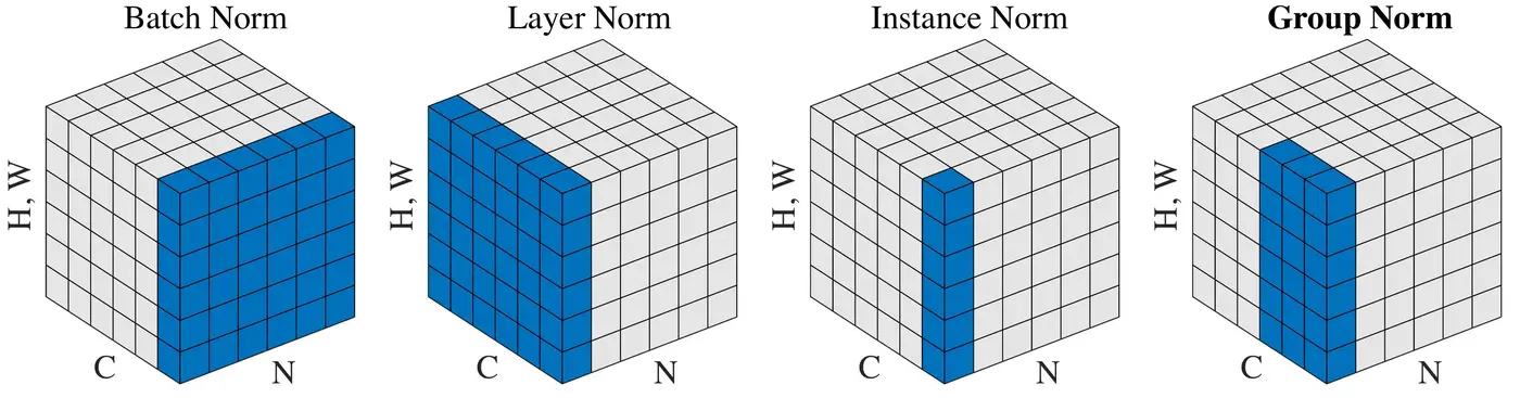
Normalization methods (Wu and He, 2018)
Batch, layer, instance and group normalization are four methods commonly used for normalizing hidden states. Their main differentiator is the dimension along which they are applied. The figure above illustrates this difference. \(N\) is the batch axis, \(C\) the channel axis, and \((H, W)\) are the spatial axes, i.e. the height and width. In fully-connected neural networks, the channel axis represents the neurons in a layer, while the spatial axes have a size of 1. In convolutional neural networks, the channel axis represents the filters in a layer while the spatial axes correspond to the filter’s height and width. Batch norm normalizes weighted sums across a mini-batch, while the other three methods operate on a single instance.
Batch Norm
Batch normalization (Ioffe and Szegedy, 2015) standardizes each hidden feature (neuron) using its mean and variance across a mini-batch. For a batch \(\mathcal{B} = x_{1…m}\) with \(m\) samples, we calculate the mean \(\mu_{\mathcal{B}}\) and variance \(\sigma_{\mathcal{B}}^2\) of each activation across the batch:
\[\mu_{\mathcal{B}} = \frac{1}{m} \sum_{i=1}^m x_i\] \[\sigma_{\mathcal{B}}^2 = \frac{1}{m} \sum_{i=1}^m (x_i - \mu_{\mathcal{B}})^2\]The activations are then normalized based on their mean and variance across the mini-batch. Essentially, we calculate their standard score, or z-score. The normalized activations \(\hat{x}_i\) are given by:
\[\hat{x}_i = \frac{x_i - \mu_{\mathcal{B}}}{\sqrt{\sigma_{\mathcal{B}}^2 + \epsilon}}\]where \(\epsilon\) is a constant used for numerical stability. The distribution of values of any \(\hat{x}\) has an expected value of \(0\) and a variance of \(1\).
Normalizing hidden units to have zero mean and unit variance restricts the representations that the model can learn. Batch normalization therefore introduces two learnable parameter vectors \(\gamma\) and \(\beta\) that shift and scale the normalized activations along the channel axis:
\[y_i = \gamma \hat{x}_i + \beta\]Applying this linear transformation on the normalized activations effectively converts the mean and variance of the hidden units into known, learnable parameters.
During inference, the activations are normalized using a moving average of the mean and variance of the mini-batches it has seen during training. These are given by:
\[\mu_{new} = \alpha \mu + (1 - \alpha) \mu_t\] \[\sigma^2_{new} = \alpha \sigma^2 + (1 - \alpha) \sigma^2_t\]where \(\mu\) and \(\sigma^2\) are the running averages, \(\mu_t\) and \(\sigma^2_t\) are the new observed values, and \(\alpha\) is a momentum parameter that is usually set to \(0.9\) or \(0.99\).
For 1D inputs (i.e. with spatial axes of size 1), batch norm can be implemented as follows:
class BatchNorm():
    """Batch Normalization"""

    def __init__(self, C, momentum=0.99):
        self.gamma = np.ones(C)
        self.beta = np.zeros(C)
        self.avg_mean = np.zeros(C)
        self.avg_var = np.ones(C)
        self.alpha = momentum

    def forward(self, x, eps=1e-8, inference=False):
        # x: input with shape (N, C)
        if inference:
            x_hat = (x - self.avg_mean) / np.sqrt(self.avg_var + eps)
            y = self.gamma * x_hat + self.beta
            return y
        mean = x.mean(axis=0, keepdims=True)
        var = x.var(axis=0, keepdims=True)
        self.avg_mean = self.alpha * self.avg_mean + (1-self.alpha) * mean
        self.avg_var = self.alpha * self.avg_var + (1-self.alpha) * var
        x_hat = (x - mean) / np.sqrt(var + eps)
        y = self.gamma * x_hat + self.beta
        return y

x = np.array([
    [1.4, 0.62, 0.21], # Sample 1
    [-.2, 1.6, -1.35], # Sample 2
    [-.97, 1.3, -2.1]  # Sample 3
])
bn = BatchNorm(C=3)
y = bn.forward(x)
y
array([[ 1.34058903, -1.34963806, 1.34069849], [-0.28027428, 1.04068477, -0.28061131], [-1.06031475, 0.30895329, -1.06008718]])
print(f"Before BN:\n{'Mean':<11}{x.mean(axis=0)}\nVariance {x.var(axis=0)}")
print(f"After BN:\n{'Mean':<11}{y.mean(axis=0)}\nVariance {y.var(axis=0)}")
Before BN: Mean [ 0.07666667 1.17333333 -1.08 ] Variance [0.97442222 0.16808889 0.9258 ] After BN: Mean [ 0.00000000e+00 -4.99600361e-16 0.00000000e+00] Variance [0.99999999 0.99999994 0.99999999]
Batch normalization can considerably improve the performance of deep neural networks. It also reduces their sensitivity to hyperparamaters such as the learning rate and the initialization strategy. One of its drawbacks is that it requires sufficiently large batch sizes (e.g. 32) to work well. Small batch sizes result in inaccurate estimations of the mean and variance of the batch and can thus lead to a higher model error. Another downside is that it relies on statistics pre-computed from the training set to perform normalization at inference time. If the data distribution changes between training and inference, this can lead to inconsistent results.
Layer Norm
Layer normalization (Ba et al., 2016) standardizes all hidden features in a layer using their mean and variance for a single training sample. All the units in a layer therefore share the same normalization terms, but different training examples have different normalization terms.
Its implementation differs from that of batch normalization in two aspects: the mean \(\mu\) and variance \(\sigma^2\) are calculated along the layer dimension, and the moving averages thereof are dispensed off. Since layer normalization does not depend on batch statistics, there is no need to calculate running averages of the mean and variance for use at inference.
For 1D inputs, layer normalization can be implemented as follows:
class LayerNorm():
    """Layer Normalization"""

    def __init__(self, C):
        # C: number of channels
        self.gamma = np.ones(C)
        self.beta = np.zeros(C)

    def forward(self, x, eps=1e-8):
        # x: input with shape (N, C)
        mean = x.mean(axis=1, keepdims=True)
        var = x.var(axis=1, keepdims=True)
        x_hat = (x - mean) / np.sqrt(var + eps)
        y = self.gamma * x_hat + self.beta
        return y

ln = LayerNorm(C=3)
y = ln.forward(x)
y
array([[ 1.3304131 , -0.24987454, -1.08053856], [-0.17846774, 1.30418734, -1.1257196 ], [-0.26877674, 1.33681063, -1.06803389]])
print(f"Before LN:\n{'Mean':<11}{x.mean(axis=1)}\nVariance {x.var(axis=1)}")
print(f"After LN:\n{'Mean':<11}{y.mean(axis=1)}\nVariance {y.var(axis=1)}")
Before LN: Mean [ 0.74333333 0.01666667 -0.59 ] Variance [0.24362222 1.47388889 1.99886667] After LN: Mean [ 0.00000000e+00 0.00000000e+00 -7.40148683e-17] Variance [0.99999996 0.99999999 0.99999999]
Layer normalization is particularly effective for training sequential models (RNN/LSTM), whose inputs vary in length for different training examples.
Instance Norm
Instance normalization (Ulyanov et al., 2017) standardizes all hidden features in a layer using their mean and variance for a single training sample and for a single channel. In models such as convolutional neural networks, where each layer results in a 3D volume of activations (H x W x C), the activations of each channel are therefore normalized independently.
# Batch of activations with 4 channels
cnn = np.array([
    # Sample 1 (H x W x C -> 2 x 2 x 4)
    [[[0.43, 0.5, 0.2, 0.4], [0.8, 0.84, 0.5, 0.7]],
     [[0.1, 0.74, 0.8, 0.2], [0.42, 0.5, 0.8, 0.6]]],
    # Sample 2
    [[[0.97, 0.7, 0.3, 0.8], [0.7, 0.13, 0.9, 0.0]],
     [[0.5, 0.8, 0.17, 0.5], [0.1, 0.86, 0.7, 0.9]]],
])
cnn.shape
(2, 2, 2, 4)
Compared to layer normalization, the only theoretical difference of instance normalization is that it normalizes each channel independently.
The implementation below is adapted for 4D inputs.
class InstanceNorm():
    """Instance Normalization"""

    def __init__(self, C):
        # C: number of channels
        self.gamma = np.ones(C)
        self.beta = np.zeros(C)

    def forward(self, x, eps=1e-8):
        # x: input with shape (N, H, W, C)
        mean = x.mean(axis=(1, 2), keepdims=True)
        var = x.var(axis=(1, 2), keepdims=True)
        x_hat = (x - mean) / np.sqrt(var + eps)
        y = self.gamma * x_hat + self.beta
        return y

inn = InstanceNorm(C=4)
y = inn.forward(cnn)
y
array([[[[-0.03026291, -0.97153634, -1.5075566 , -0.39056668], [ 1.4627075 , 1.30654887, -0.30151132, 1.17170004]], [[-1.36183112, 0.63652381, 0.90453396, -1.43207783], [-0.07061347, -0.97153634, 0.90453396, 0.65094447]]], [[[ 1.26858194, 0.26721158, -0.73773859, 0.71428569], [ 0.41760772, -1.69808648, 1.29740234, -1.57142851]], [[-0.21274356, 0.61200071, -1.17868579, -0.14285714], [-1.47344611, 0.81887419, 0.61902203, 0.99999996]]]])
print(f"Before IN:\n{'Mean':<11}{cnn.mean(axis=(1, 2))}\nVariance {cnn.var(axis=(1, 2))}")
print(f"After IN:\n{'Mean':<11}{y.mean(axis=(1, 2))}\nVariance {y.var(axis=(1, 2))}")
Before IN: Mean [[0.4375 0.645 0.575 ] [0.5675 0.6225 0.515 ]] Variance [[0.06141875 0.022275 0.061875 ] [0.10066875 0.08411875 0.085025 ]] After IN: Mean [[-6.93889390e-18 -1.66533454e-16 2.77555756e-16] [-5.55111512e-17 1.94289029e-16 3.05311332e-16]] Variance [[0.99999984 0.99999955 0.99999984] [0.9999999 0.99999988 0.99999988]]
Empirical evidence suggests that instance normalization works well as a replacement for batch normalization in GANs and for neural style transfer.
Group Norm
Group normalization (Wu and He, 2018) is a generalization of single instance normalization methods to any group of channels. Layer normalization computes statistics across all channels, while instance normalization does so for each channel. Group normalization extends these methods to any division of the channels. Layer and instance normalization can therefore be seen as specific cases of group normalization.
The motivation behind group normalization is that features such as the filters of convolutional neural networks are group-wise representations (i.e. they are interrelated) and should therefore be normalized as such.
class GroupNorm():
    """Group Normalization"""

    def __init__(self, C):
        # C: number of channels
        self.gamma = np.ones(C)
        self.beta = np.zeros(C)

    def forward(self, x, G, eps=1e-8):
        # x: input with shape (N, H, W, C)
        # G: number of groups
        N, H, W, C = x.shape
        x = x.reshape(N, H, W, G, C // G)
        mean = x.mean(axis=(1, 2, 4), keepdims=True)
        var = x.var(axis=(1, 2, 4), keepdims=True)
        x_hat = (x - mean) / np.sqrt(var + eps)
        x_hat = x_hat.reshape(N, H, W, C)
        y = self.gamma * x_hat + self.beta
        return y

gn = GroupNorm(C=4)
y = gn.forward(cnn, G=2)
y
array([[[[-0.48502258, -0.17983983, -1.42693524, -0.54882125], [ 1.12808623, 1.30247637, -0.10976425, 0.76834975]], [[-1.92374125, 0.86650101, 1.20740674, -1.42693524], [-0.52862012, -0.17983983, 1.20740674, 0.32929275]]], [[[ 1.2286829 , 0.34403121, -0.72145939, 0.82176925], [ 0.34403121, -1.5235668 , 1.13041498, -1.64739657]], [[-0.31126634, 0.67167999, -1.12269883, -0.10416793], [-1.62186143, 0.86826925, 0.51312352, 1.13041498]]]])
eval_cnn = cnn.reshape((2, 2, 2, 2, 2))
eval_y = y.reshape((2, 2, 2, 2, 2))

print(f"Before GN:\n{'Mean':<11}{eval_cnn.mean(axis=(1, 2, 4))}\nVariance {eval_cnn.var(axis=(1, 2, 4))}")
print(f"After GN:\n{'Mean':<11}{eval_y.mean(axis=(1, 2, 4))}\nVariance {eval_y.var(axis=(1, 2, 4))}")
Before GN: Mean [[0.54125 0.525 ] [0.595 0.53375]] Variance [[0.05261094 0.051875 ] [0.09315 0.10497344]] After GN: Mean [[-1.11022302e-16 4.44089210e-16] [ 8.32667268e-17 2.22044605e-16]] Variance [[0.99999981 0.99999981] [0.99999989 0.9999999 ]]
Wu and He (2018) report that group normalization achieves better results than batch normalization in ResNets with low batch sizes, and similar results when using normal batch sizes.
Assembling the Building Blocks Together
The challenge of deep learning lies in assembling and optimizing models to solve a specific problem. In this last section, we build and train a fully-connected neural network for the task of recognizing handwritten digits.
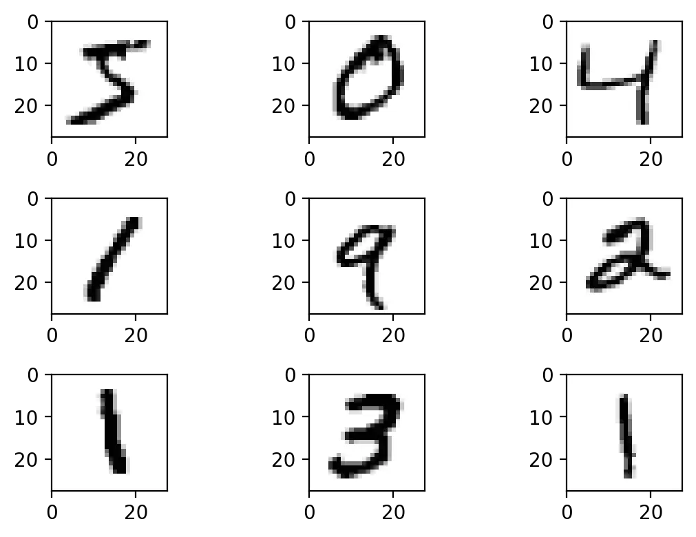
MNIST
The MNIST dataset, assembled by LeCun et al. (1998a), is a collection of binary images of handwritten digits. The digits are size-normalized and centered in images of size 28x28. The dataset consists of a training set of 60,000 samples, a test set of 10,000 samples, and their corresponding labels.
MNIST is a classic dataset in machine learning, and is often used in introductions to the field owing to its simplicity and the ease of training different classifiers on it.
(X_train, y_train), (X_test, y_test) = mnist.load_data()
X_train.shape
(60000, 28, 28)
The grayscale images have a pixel depth of 256, i.e. pixel values ranging from 0 to 255. We rescale the pixel values so that they range between 0 and 1.
X_train = X_train.astype("float32") / 255
X_test = X_test.astype("float32") / 255
Since we’ll train fully-connected neural networks, we flatten each image into a single dimension.
X_train = X_train.reshape((60000, 784))
X_test = X_test.reshape((10000, 784))
Next, the labels are encoded as one-hot encoded vectors to match the output of the neural network.
def onehot(y):
    """Encodes the expected result as a one-hot vector"""
    v = np.zeros((y.size, y.max()+1))
    v[np.arange(y.size), y] = 1
    return v

# Example
onehot(np.array([5, 0, 9]))
array([[0., 0., 0., 0., 0., 1., 0., 0., 0., 0.], [1., 0., 0., 0., 0., 0., 0., 0., 0., 0.], [0., 0., 0., 0., 0., 0., 0., 0., 0., 1.]])
y_train = onehot(y_train)
y_test = onehot(y_test)
Our neural network consists of single hidden layer with 600 units and ReLU activations followed by an output layer with 10 units and softmax activations. The loss is given by the cross-entropy loss function. We also apply weight decay (L2 normalization) to the weights of the hidden and output layer.
For the backward pass, we backpropagate the loss through the loss function and output layer by taking the partial derivative of the cross-entropy function with respect to the weighted sum \(z\) of the output layer. Since the output of the network \(\hat{y}\) is given by \(softmax(z)\) and the loss \(L\) by \(CE(y, \hat{y})\):
\[\frac{\partial L}{\partial z} = \hat{y} - y\]class NeuralNetwork:
def __init__(self):
# Input layer: 784 inputs
# Hidden layer: 600 neurons
self.w1 = he(inputs=784, neurons=600)
self.b1 = np.zeros((1, 600))
# Output layer: 10 neurons
self.w2 = xavier(inputs=600, neurons=10)
self.b2 = np.zeros((1, 10))
def forward(self, x):
"""Forward pass"""
a1 = relu(x @ self.w1 + self.b1)
pred = softmax(a1 @ self.w2 + self.b2)
return pred
def backprop(self, X, y, lmbda):
"""Compute gradient over the batch through backpropagation
Inputs:
- X: batch of inputs
- y: batch of labels
- lmbda: weight decay parameter
"""
# Forward pass, caching intermediate values
z1 = X @ self.w1 + self.b1
a1 = relu(z1)
z2 = a1 @ self.w2 + self.b2
pred = softmax(z2)
# Cross-entropy loss with L2 regularization
loss = cross_entropy(y, pred)
loss += lmbda * (np.sum(self.w1**2) + np.sum(self.w2**2))
# Backward pass
dL_dz2 = pred - y
dL_dw2 = a1.T @ dL_dz2 / len(X)
dL_db2 = np.mean(dL_dz2, axis=0, keepdims=True)
dL_da1 = dL_dz2 @ self.w2.T
dL_dz1 = dL_da1 * relu(z1, derivative=True)
dL_dw1 = X.T @ dL_dz1 / len(X)
dL_db1 = np.mean(dL_dz1, axis=0, keepdims=True)
return loss, (dL_dw1, dL_dw2, dL_db1, dL_db2)
def evaluate(self, X, y):
"""Evaluate the accuracy of the model"""
preds = model.forward(X)
acc = sum(np.argmax(preds, axis=1) == np.argmax(y, axis=1)) / len(y)
return acc
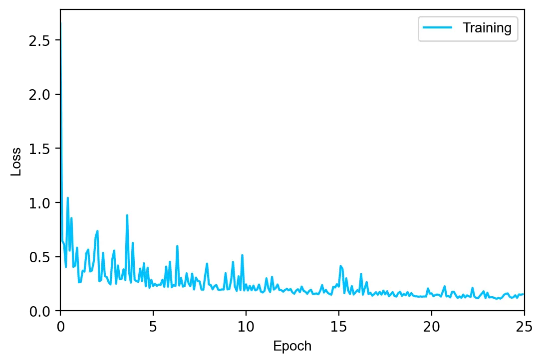
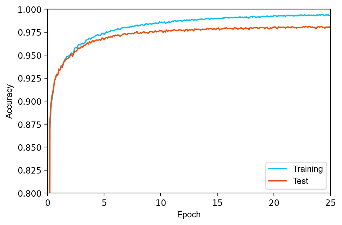
We train the model using mini-batch SGD for a total of 25 epochs. The learning rate is set to \(0.02\), the batch size to \(16\) and the regularization parameter \(\lambda\) to \(0.0002\).
model = NeuralNetwork()
epochs = 25
lr = 0.02
batch_size = 16
lmbda = 2e-4

for epoch in range(epochs):
    X_train, y_train = shuffle(X_train, y_train)
    for i in range(0, len(X_train), batch_size):
        X = X_train[i:i+batch_size]
        y = y_train[i:i+batch_size]
        loss, grads = model.backprop(X, y, lmbda)
        dL_dw1, dL_dw2, dL_db1, dL_db2 = grads
        model.w1 -= lr * (dL_dw1 + 2 * lmbda * model.w1)
        model.b1 -= lr * dL_db1
        model.w2 -= lr * (dL_dw2 + 2 * lmbda * model.w2)
        model.b2 -= lr * dL_db2
    if epoch % 2 == 0:
        train_acc = model.evaluate(X_train, y_train)
        test_acc = model.evaluate(X_test, y_test)
        print(f"loss: {loss:.4f} train acc.: {train_acc:.4f} test acc.: {test_acc:.4f} [{epoch+1:>2d}/{epochs}]")
loss: 0.7563 train acc.: 0.9346 test acc.: 0.9342 [ 1/25] loss: 0.2384 train acc.: 0.9626 test acc.: 0.9586 [ 3/25] loss: 0.4797 train acc.: 0.9740 test acc.: 0.9686 [ 5/25] loss: 0.2492 train acc.: 0.9805 test acc.: 0.9734 [ 7/25] loss: 0.2081 train acc.: 0.9839 test acc.: 0.9757 [ 9/25] loss: 0.1762 train acc.: 0.9864 test acc.: 0.9771 [11/25] loss: 0.1604 train acc.: 0.9886 test acc.: 0.9783 [13/25] loss: 0.1501 train acc.: 0.9901 test acc.: 0.9803 [15/25] loss: 0.2813 train acc.: 0.9909 test acc.: 0.9799 [17/25] loss: 0.1618 train acc.: 0.9923 test acc.: 0.9802 [19/25] loss: 0.1423 train acc.: 0.9930 test acc.: 0.9804 [21/25] loss: 0.1826 train acc.: 0.9939 test acc.: 0.9811 [23/25] loss: 0.2321 train acc.: 0.9943 test acc.: 0.9815 [25/25]
The model achieves a test error of 1.85%, in line with other fully-connected neural networks of similar size. Despite L2 regularization, the training and test accuracy differ by 1.28%, indicating that the model slightly overfits on the training set.
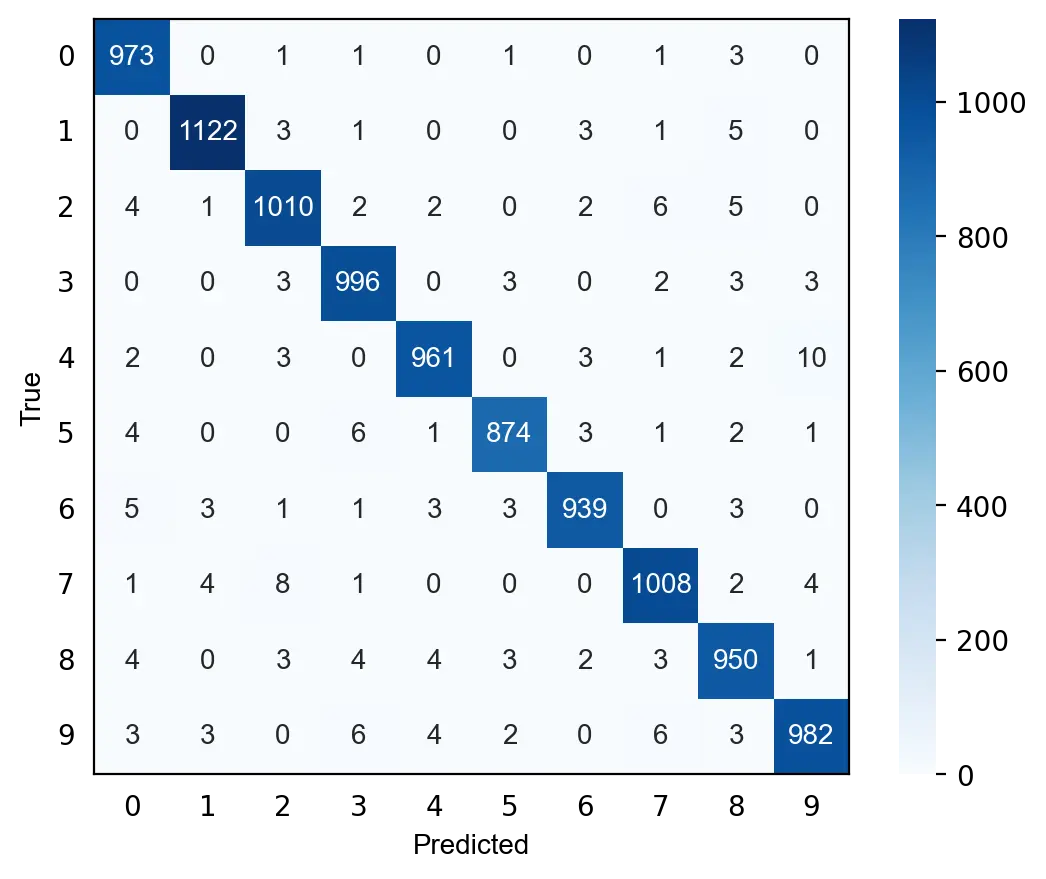
We can also evaluate the model by visualizing its predictions on the test set with a confusion matrix. As can be seen below, digits such as 0, 1 and 3 are seldom misclassified while other such 8 and 9 are misclassified more frequently. The model particularly struggles with distinguishing between 4 and 9, and between 2 and 7.
Pytorch
Defining and integrating all building blocks of a neural network by hand is slow and error-prone. The complexity of doing so increases with the number of layers and when using optimizers other than mini-batch SGD. Deep learning libraries such as Pytorch simplify this task by providing an API to define models, automatic differentation, primitives to handle and load data, and support for accelerators such as GPUs.
For comparison, we define the same model in Pytorch. Note that the softmax activation function is omitted from the model definition because it is included in Pytorch’s CrossEntropyLoss function.
class PytorchNeuralNetwork(nn.Module):

    def __init__(self):
        super(PytorchNeuralNetwork, self).__init__()
        self.layers = nn.Sequential(
            nn.Linear(784, 600),
            nn.ReLU(),
            nn.Linear(600, 10)
        )

    def forward(self, x):
        pred = self.layers(x)
        return pred

    def evaluate(self, x, y):
        preds = model.forward(x)
        acc = sum(torch.argmax(preds, 1) == torch.argmax(y, 1)) / len(y)
        return acc
Pytorch provides two primitives for handling data: torch.utils.data.Dataset and torch.utils.data.DataLoader. Dataset stores the samples and their corresponding labels while DataLoader creates an iterable over an instance of Dataset.
First, we convert the data into torch tensors.
X_train = torch.tensor(X_train, dtype=torch.float)
X_test = torch.tensor(X_test, dtype=torch.float)
y_train = torch.tensor(y_train, dtype=torch.float)
y_test = torch.tensor(y_test, dtype=torch.float)

X_train.shape
torch.Size([60000, 784])
Next, we load the training data into TensorDataset, a subclass of Dataset, and wrap it with DataLoader.
train_data = TensorDataset(X_train, y_train)
train_loader = DataLoader(train_data, batch_size=32, shuffle=True)
The model is trained for \(30\) epochs using the Adam optimizer with a learning rate of \(0.0002\). Since the previous model was slightly overfitted, we increase the regularization parameter \(\lambda\) to \(0.003\).
model = PytorchNeuralNetwork().to("cpu")
loss_fn = nn.CrossEntropyLoss()
optimizer = torch.optim.Adam(model.parameters(), lr=2e-4, weight_decay=1e-3)
epochs = 30

# Training loop
for epoch in range(epochs):
    for i, (inputs, labels) in enumerate(train_loader):
        # Forward pass
        pred = model.forward(inputs)
        loss = loss_fn(pred, labels)
        # Backward pass
        optimizer.zero_grad()
        loss.backward()
        optimizer.step()
    if (epoch+1) % 2 == 0:
        train_acc = model.evaluate(X_train, y_train)
        test_acc = model.evaluate(X_test, y_test)
        print(f"loss: {loss.data:.4f} train acc.: {train_acc:.4f} test acc.: {test_acc:.4f} [{epoch+1:>2d}/{epochs}]")
loss: 0.1298 train acc.: 0.9578 test acc.: 0.9546 [ 2/30] loss: 0.0853 train acc.: 0.9711 test acc.: 0.9668 [ 4/30] loss: 0.0920 train acc.: 0.9783 test acc.: 0.9716 [ 6/30] loss: 0.0307 train acc.: 0.9812 test acc.: 0.9754 [ 8/30] loss: 0.0546 train acc.: 0.9815 test acc.: 0.9739 [10/30] loss: 0.1141 train acc.: 0.9845 test acc.: 0.9782 [12/30] loss: 0.0280 train acc.: 0.9840 test acc.: 0.9777 [14/30] loss: 0.1350 train acc.: 0.9845 test acc.: 0.9772 [16/30] loss: 0.1357 train acc.: 0.9837 test acc.: 0.9760 [18/30] loss: 0.2754 train acc.: 0.9851 test acc.: 0.9768 [20/30] loss: 0.0129 train acc.: 0.9868 test acc.: 0.9792 [22/30] loss: 0.0308 train acc.: 0.9866 test acc.: 0.9772 [24/30] loss: 0.0408 train acc.: 0.9842 test acc.: 0.9769 [26/30] loss: 0.0939 train acc.: 0.9868 test acc.: 0.9791 [28/30] loss: 0.1069 train acc.: 0.9853 test acc.: 0.9769 [30/30]
While the Pytorch model has a smaller generalization gap than the previous model, it performs slightly worse. The Pytorch model achieves a maximum test accuracy of 97.92% (error of 2.08%), compared to 98.15% for the previous model. This could be due to the initialization, the different optimizer, or the stronger regularization.
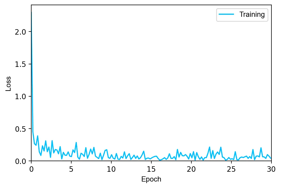
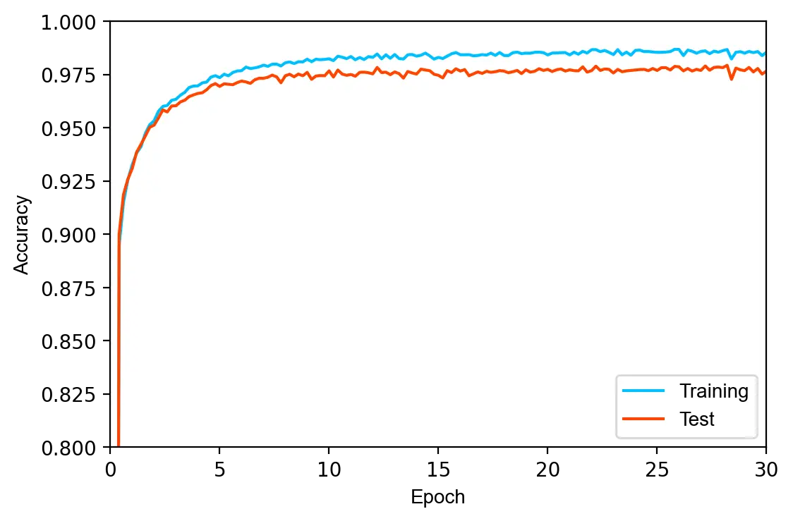
Further hyperparameter tuning will likely only lead to marginal improvements. Instead, a new architecture such as a CNN, dataset augmentation, and an increased representational capacity are more likely to improve the test set accuracy. State of the art models have an accuracy of over 95.5% on the MNIST dataset. LeCun (1998) has compiled an overview of several approaches and their results, while Papers with Code provides a benchmark of the top recent methods.
References
- Action potential - Wikipedia. (n.d.). Retrieved March 31, 2022, from https://en.wikipedia.org/wiki/Action_potential
- Ba, J. L., Kiros, J. R., & Hinton, G. E. (2016). Layer Normalization. https://doi.org/10.48550/arxiv.1607.06450
- Baydin, A. G., Pearlmutter, B. A., Radul, A. A., & Siskind, J. M. (2018). Automatic Differentiation in Machine Learning: a Survey. Journal of Machine Learning Research, 18(153), 1–43. http://jmlr.org/papers/v18/17-468.html
- Chollet, F. (2021). Deep Learning with Python (2nd Ed.). Manning.
- CS231n Convolutional Neural Networks for Visual Recognition. (2022). https://cs231n.github.io/
- Duchi, J., Hazan, E., & Singer, Y. (2011). Adaptive Subgradient Methods for Online Learning and Stochastic Optimization. Journal of Machine Learning Research, 12, 2121–2159.
- Glorot, X., & Bengio, Y. (2010). Understanding the difficulty of training deep feedforward neural networks. In Y. W. Teh & M. Titterington (Eds.), Proceedings of the Thirteenth International Conference on Artificial Intelligence and Statistics (Vol. 9, pp. 249–256). PMLR. https://proceedings.mlr.press/v9/glorot10a.html
- Goodfellow, I., Bengio, Y., & Courville, A. (2016). Deep Learning. MIT Press.
- Hinton, G. (2012). Neural Networks for Machine Learning Lecture 6a Overview of mini--batch gradient descent. https://www.cs.toronto.edu/~tijmen/csc321/slides/lecture_slides_lec6.pdf
- Ioffe, S., & Szegedy, C. (2015). Batch Normalization: Accelerating Deep Network Training by Reducing Internal Covariate Shift. 32nd International Conference on Machine Learning, ICML 2015, 1, 448–456. https://doi.org/10.48550/arxiv.1502.03167
- Kingma, D. P., & Ba, J. L. (2014). Adam: A Method for Stochastic Optimization. 3rd International Conference on Learning Representations, ICLR 2015 - Conference Track Proceedings. https://doi.org/10.48550/arxiv.1412.6980
- Murphy, K. P. (2022). Probabilistic Machine Learning: An introduction. MIT Press.
- Nielsen, M. A. (2015). Neural Networks and Deep Learning. Determination Press.
- Ruder, S. (2016). An overview of gradient descent optimization algorithms. arXiv. https://doi.org/10.48550/arxiv.1609.04747
- Srivastava, N., Hinton, G., Krizhevsky, A., Sutskever, I., & Salakhutdinov, R. (2014). Dropout: A Simple Way to Prevent Neural Networks from Overfitting. Journal of Machine Learning Research, 15(56), 1929–1958. http://jmlr.org/papers/v15/srivastava14a.html
- Ulyanov, D., Vedaldi, A., & Lempitsky, V. (2016). Instance Normalization: The Missing Ingredient for Fast Stylization. https://doi.org/10.48550/arxiv.1607.08022
- Wu, Y., & He, K. (2018). Group Normalization. International Journal of Computer Vision, 128(3), 742–755. https://doi.org/10.48550/arxiv.1803.08494